Quality Control on in-silico spatial proteomics with Harpy

Introduction

This noteboook outlines some quality controls steps for highly-multiplexed spatial proteomics data using the Harpy package. Most steps are similar to this good resource on Imaging Mass Cytometry data analysis in R from the Bodenmiller lab. Here, an artificial in-silico dataset is used to demonstrate the quality control steps.

The levels of quality control are:

• Image level: to give an overview of the quality of the images in the dataset.

• Segmentation level: to give an overview of the quality of the segmentation in the dataset.

• Cell level: to give an overview of the quality of the calculated features per cell in the dataset.

We start by loading in an example dataset and visualising the data:

import harpy
import matplotlib.pyplot as plt
import spatialdata_plot  # noqa
import scanpy as sc
from harpy.datasets import multisample_blobs

plt.viridis()

sdata = multisample_blobs(n_samples=4)
sdata

The autoreload extension is already loaded. To reload it, use:
  %reload_ext autoreload
INFO     no axes information specified in the object, setting `dims` to: ('c', 'y', 'x')                           
INFO     no axes information specified in the object, setting `dims` to: ('y', 'x')
INFO     no axes information specified in the object, setting `dims` to: ('c', 'y', 'x')                           
INFO     no axes information specified in the object, setting `dims` to: ('y', 'x')
INFO     no axes information specified in the object, setting `dims` to: ('c', 'y', 'x')                           
INFO     no axes information specified in the object, setting `dims` to: ('y', 'x')
INFO     no axes information specified in the object, setting `dims` to: ('c', 'y', 'x')                           
INFO     no axes information specified in the object, setting `dims` to: ('y', 'x')

SpatialData object
├── Images
│     ├── 'sample_0_image': DataArray[cyx] (11, 512, 512)
│     ├── 'sample_1_image': DataArray[cyx] (11, 512, 512)
│     ├── 'sample_2_image': DataArray[cyx] (11, 512, 512)
│     └── 'sample_3_image': DataArray[cyx] (11, 512, 512)
├── Labels
│     ├── 'sample_0_labels': DataArray[yx] (512, 512)
│     ├── 'sample_1_labels': DataArray[yx] (512, 512)
│     ├── 'sample_2_labels': DataArray[yx] (512, 512)
│     └── 'sample_3_labels': DataArray[yx] (512, 512)
├── Points
│     ├── 'sample_0_points': DataFrame with shape: (<Delayed>, 2) (2D points)
│     ├── 'sample_1_points': DataFrame with shape: (<Delayed>, 2) (2D points)
│     ├── 'sample_2_points': DataFrame with shape: (<Delayed>, 2) (2D points)
│     └── 'sample_3_points': DataFrame with shape: (<Delayed>, 2) (2D points)
└── Tables
      ├── 'sample_0_table': AnnData (20, 11)
      ├── 'sample_1_table': AnnData (20, 11)
      ├── 'sample_2_table': AnnData (20, 11)
      ├── 'sample_3_table': AnnData (20, 11)
      └── 'table': AnnData (80, 11)
with coordinate systems:
    ▸ 'sample_0', with elements:
        sample_0_image (Images), sample_0_labels (Labels), sample_0_points (Points)
    ▸ 'sample_1', with elements:
        sample_1_image (Images), sample_1_labels (Labels), sample_1_points (Points)
    ▸ 'sample_2', with elements:
        sample_2_image (Images), sample_2_labels (Labels), sample_2_points (Points)
    ▸ 'sample_3', with elements:
        sample_3_image (Images), sample_3_labels (Labels), sample_3_points (Points)

<Figure size 640x480 with 0 Axes>

table = sdata["table"]

table.to_df()

	nucleus	lineage_0	lineage_1	lineage_2	lineage_3	lineage_4	lineage_5	lineage_6	lineage_7	lineage_8	lineage_9
cells
1	130579.074583	73143.384718	90176.329291	78887.342227	83547.398858	0.000000	85104.954042	89203.618952	71052.452962	166453.784109	79783.723973
2	97747.257070	44127.352051	54403.315415	47592.677537	50404.086393	0.000000	51343.758329	103611.315408	42865.894408	48557.293269	48133.464008
3	129783.693347	72871.920340	89159.713324	77997.994298	82605.515103	0.000000	132335.765591	88197.968976	70251.432797	79581.243727	78884.270554
4	126967.536598	69764.494608	86010.594981	159287.142678	79687.890840	0.000000	81180.370216	85082.819414	67770.154343	76768.146443	76776.118424
5	107214.353348	52460.254002	64676.705321	56579.963133	124573.992918	0.000000	61039.388909	63979.053282	50960.585762	57726.734557	57222.870407
...	...	...	...	...	...	...	...	...	...	...	...
16	161696.495625	84635.637309	175638.724282	105850.500384	102504.128585	88371.831230	106509.552476	97690.881838	97966.012854	96128.415489	0.000000
17	163295.271990	86338.942986	93873.258186	107784.066049	104567.040494	90150.328405	108653.074179	188483.571632	99937.594462	98063.015157	0.000000
18	153201.459416	75869.389265	82490.085245	94714.053483	91887.127930	80816.560758	95477.684746	87572.419579	175560.397181	86171.787748	0.000000
19	154421.629069	153238.714827	83799.306745	96217.284748	93345.492327	80475.900902	96993.035800	88962.304123	89212.852472	88883.535945	0.000000
20	161275.579840	84186.643485	175348.640010	105097.641133	101960.342041	87903.016819	105944.517075	97172.629669	97446.301109	95618.452236	0.000000

80 rows × 11 columns

table.var

	cycle
nucleus	0
lineage_0	0
lineage_1	1
lineage_2	1
lineage_3	2
lineage_4	2
lineage_5	3
lineage_6	3
lineage_7	4
lineage_8	4
lineage_9	5

table.obs

	instance_id	region	fov_labels	cell_ID	phenotype	area	eccentricity	major_axis_length	minor_axis_length	perimeter	centroid-0	centroid-1	convex_area	equivalent_diameter	_major_minor_axis_ratio	_perim_square_over_area	_major_axis_equiv_diam_ratio	_convex_hull_resid	_centroid_dif
cells
1	1	by	sample_0_labels	1	8	2393.0	0.000000	55.199096	55.199096	180.852814	482.000000	410.000000	2433.0	55.198390	1.000000	13.668090	1.000013	0.016441	0.000000
2	2	by	sample_0_labels	2	6	1489.0	0.840912	60.858245	32.934784	160.083261	161.000000	12.721961	1519.0	43.541402	1.847841	17.210645	1.397710	0.019750	0.003520
3	3	by	sample_0_labels	3	5	2332.0	0.296286	55.821777	53.315330	179.338095	369.522298	388.423671	2375.0	54.490317	1.047012	13.791661	1.024435	0.018105	0.001060
4	4	by	sample_0_labels	4	2	2352.0	0.249266	55.649195	53.892628	180.852814	64.180697	106.579082	2397.0	54.723481	1.032594	13.906352	1.016916	0.018773	0.001168
5	5	by	sample_0_labels	5	3	1706.0	0.765745	59.549068	38.298639	166.083261	216.000000	495.966002	1734.0	46.606294	1.554861	16.168611	1.277704	0.016148	0.002416
...	...	...	...	...	...	...	...	...	...	...	...	...	...	...	...	...	...	...	...
16	16	by	sample_3_labels	16	1	2856.0	0.198505	60.937241	59.724580	198.409163	328.041317	117.297969	2911.0	60.302339	1.020304	13.783682	1.010529	0.018894	0.001298
17	17	by	sample_3_labels	17	6	2885.0	0.000000	60.607577	60.607577	197.823376	245.000000	470.000000	2933.0	60.607723	1.000000	13.564675	0.999998	0.016365	0.000000
18	18	by	sample_3_labels	18	7	2616.0	0.508391	62.616366	53.920614	194.793939	110.995413	406.372706	2680.0	57.713037	1.161270	14.504847	1.084961	0.023881	0.003410
19	19	by	sample_3_labels	19	0	2665.0	0.466229	62.247488	55.068120	193.036580	227.496060	153.503940	2703.0	58.251038	1.130372	13.982409	1.068607	0.014058	0.001451
20	20	by	sample_3_labels	20	1	2844.0	0.237913	61.101562	59.347125	196.509668	27.427215	169.000000	2890.0	60.175520	1.029562	13.578077	1.015389	0.015917	0.000612

80 rows × 19 columns

selected_markers = table.var_names[:3].tolist()
selected_markers

['nucleus', 'lineage_0', 'lineage_1']

sdata.pl.render_images(channel=selected_markers).pl.render_labels().pl.show()

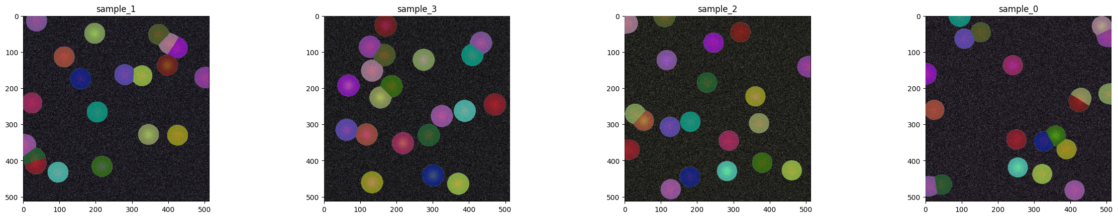
Image level quality control

table.var["cycle"]

nucleus      0
lineage_0    0
lineage_1    1
lineage_2    1
lineage_3    2
lineage_4    2
lineage_5    3
lineage_6    3
lineage_7    4
lineage_8    4
lineage_9    5
Name: cycle, dtype: int64

df = harpy.pl.calculate_snr_ratio(sdata, cycles="cycle")
df

	image	cycle	channel	snr	signal
0	sample_0_image	0	nucleus	3.287837	73.395618
1	sample_0_image	0	lineage_0	3.350054	60.223873
2	sample_0_image	1	lineage_1	3.341242	71.868568
3	sample_0_image	1	lineage_2	3.339835	62.863215
4	sample_0_image	2	lineage_3	3.341236	66.354626
5	sample_0_image	2	lineage_4	NaN	NaN
6	sample_0_image	3	lineage_5	3.328766	68.452983
7	sample_0_image	3	lineage_6	3.333190	71.719604
8	sample_0_image	4	lineage_7	3.341090	56.638927
9	sample_0_image	4	lineage_8	3.346352	65.247809
10	sample_0_image	5	lineage_9	3.351038	65.531110
11	sample_1_image	0	nucleus	3.317217	68.429706
12	sample_1_image	0	lineage_0	3.354614	57.989819
13	sample_1_image	1	lineage_1	3.347276	68.978197
14	sample_1_image	1	lineage_2	3.353919	63.870013
15	sample_1_image	2	lineage_3	3.345361	55.801995
16	sample_1_image	2	lineage_4	3.340518	72.187184
17	sample_1_image	3	lineage_5	3.348367	66.388941
18	sample_1_image	3	lineage_6	3.345955	63.479419
19	sample_1_image	4	lineage_7	3.345319	63.756732
20	sample_1_image	4	lineage_8	3.354425	67.277019
21	sample_1_image	5	lineage_9	3.351014	68.710552
22	sample_2_image	0	nucleus	3.285106	72.556726
23	sample_2_image	0	lineage_0	3.346338	66.941166
24	sample_2_image	1	lineage_1	3.348429	58.152628
25	sample_2_image	1	lineage_2	3.354761	64.411135
26	sample_2_image	2	lineage_3	3.342676	62.753927
27	sample_2_image	2	lineage_4	3.343551	62.706414
28	sample_2_image	3	lineage_5	3.346515	65.341556
29	sample_2_image	3	lineage_6	3.346694	68.759239
30	sample_2_image	4	lineage_7	3.340821	65.563372
31	sample_2_image	4	lineage_8	3.342025	63.964066
32	sample_2_image	5	lineage_9	3.342700	61.233602
33	sample_3_image	0	nucleus	3.409306	74.062011
34	sample_3_image	0	lineage_0	3.354025	59.879868
35	sample_3_image	1	lineage_1	3.355139	65.147514
36	sample_3_image	1	lineage_2	3.346811	72.394797
37	sample_3_image	2	lineage_3	3.345158	69.136590
38	sample_3_image	2	lineage_4	3.347905	60.523140
39	sample_3_image	3	lineage_5	3.344262	71.837665
40	sample_3_image	3	lineage_6	3.349851	66.981595
41	sample_3_image	4	lineage_7	3.344799	66.048378
42	sample_3_image	4	lineage_8	3.351530	66.949340
43	sample_3_image	5	lineage_9	NaN	NaN

df = df.groupby(["image", "channel"]).mean(numeric_only=True)

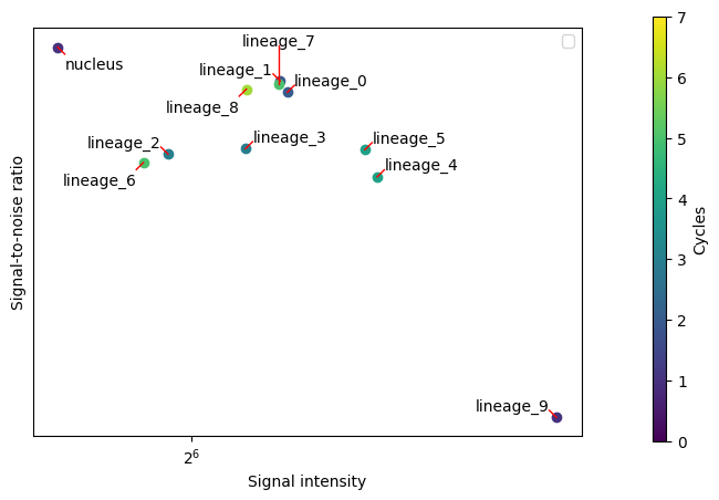
harpy.pl.snr_ratio(sdata, color="cycle")

<Axes: xlabel='Signal intensity', ylabel='Signal-to-noise ratio'>

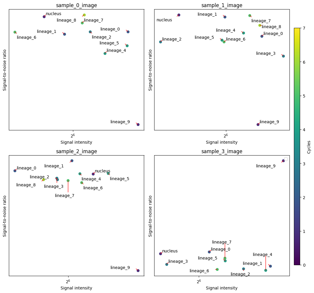
harpy.pl.group_snr_ratio(sdata, groupby=["image", "channel"], color="cycle")

array([[<Axes: title={'center': 'sample_0_image'}, xlabel='Signal intensity', ylabel='Signal-to-noise ratio'>,
        <Axes: title={'center': 'sample_1_image'}, xlabel='Signal intensity', ylabel='Signal-to-noise ratio'>],
       [<Axes: title={'center': 'sample_2_image'}, xlabel='Signal intensity', ylabel='Signal-to-noise ratio'>,
        <Axes: title={'center': 'sample_3_image'}, xlabel='Signal intensity', ylabel='Signal-to-noise ratio'>]],
      dtype=object)

harpy.pl.snr_ratio(sdata, signal_threshold=2)

<Axes: xlabel='Signal intensity', ylabel='Signal-to-noise ratio'>

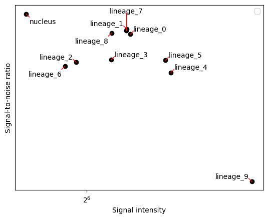
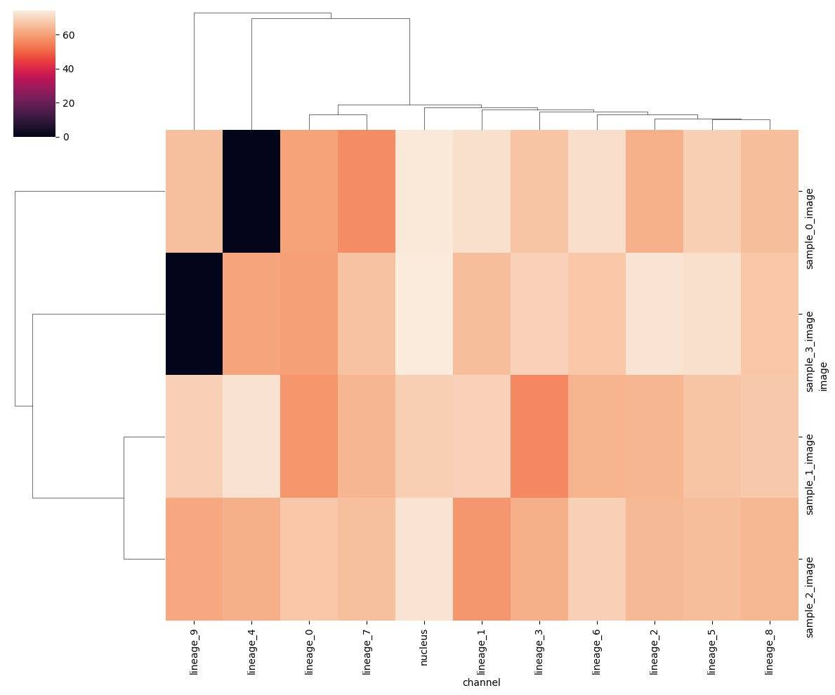
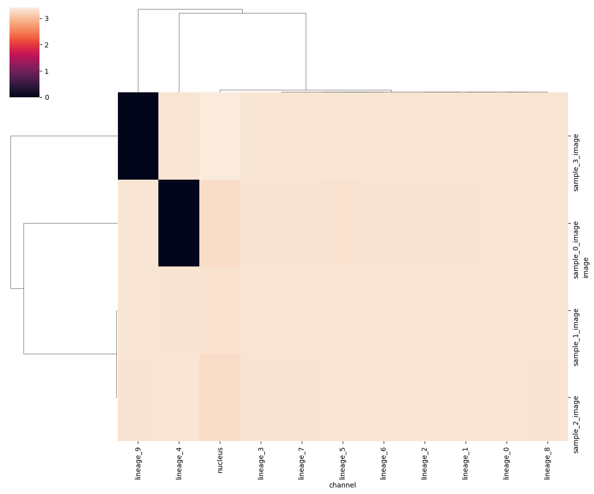
The plots above summarize all samples together. It would be interesting to look without cell segmentation bias across all channels and samples. There are multiple ways to aggregate the channel signal on an image level to a heatmap. One way is to create heatmaps using the SNR and signal values calculated above. This again depends on the unsupervised Otsu thresholding and is not a very good proxy of a good cell segmentation.

When showing the heatmap you could use the z_score or standard_scale options, but it’s also interesting not to transform the data too much in order to still visualize the outliers.

harpy.pl.signal_clustermap(sdata, signal_threshold=2, figsize=(12, 10))

<seaborn.matrix.ClusterGrid at 0x37bb615d0>

harpy.pl.snr_clustermap(sdata, signal_threshold=2, figsize=(12, 10))

<seaborn.matrix.ClusterGrid at 0x37cd5d600>

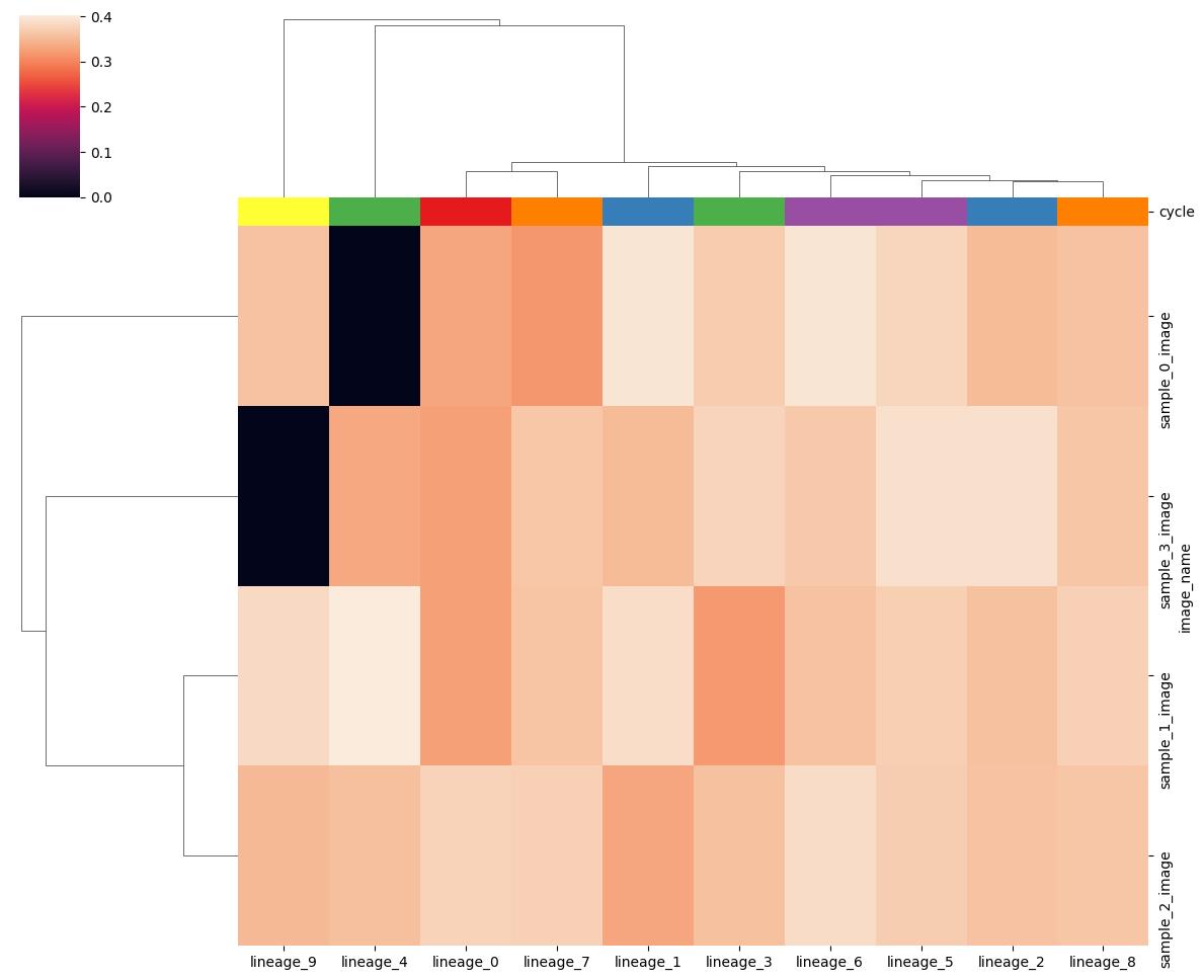
Another way is to normalize the image with a quartile normalization. The min and max quartile can greatly influence how the ends of the intensity distributions. Here we clip the signal below and above the 5th and 95th percentile. We also apply an arcsinh transformation to each channel against extreme outliers to make the heatmap more interpretable.

df_norm = harpy.pl.calculate_mean_norm(
    sdata, overwrite=True, q_min=5, q_max=95, c_mask=selected_markers[0]
)
df_norm

	lineage_0	lineage_1	lineage_2	lineage_3	lineage_4	lineage_5	lineage_6	lineage_7	lineage_8	lineage_9
image_name
sample_0_image	0.331322	0.395357	0.350663	0.368848	0.000000	0.379894	0.395442	0.316976	0.359809	0.359169
sample_1_image	0.325366	0.387694	0.357238	0.318276	0.402458	0.372283	0.359916	0.361338	0.373854	0.383336
sample_2_image	0.376520	0.330558	0.358838	0.357882	0.356515	0.370799	0.385876	0.373850	0.362120	0.349794
sample_3_image	0.323949	0.350711	0.391374	0.378530	0.332451	0.391408	0.365116	0.363468	0.362484	0.000000

# harpy.pl.clustermap(df_norm, row_colors=harpy.pl.make_cols_colors(df_metadata), figsize=(12, 10))
harpy.pl.clustermap(
    df_norm, col_colors=harpy.pl.make_cols_colors(table.var), figsize=(12, 10)
)

<seaborn.matrix.ClusterGrid at 0x37ce4b4f0>

Segmentation level quality control

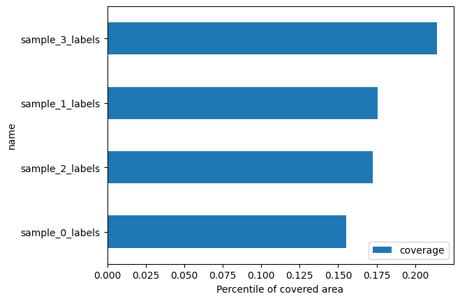
harpy.pl.segmentation_coverage(sdata)

<Axes: xlabel='Percentile of covered area', ylabel='name'>

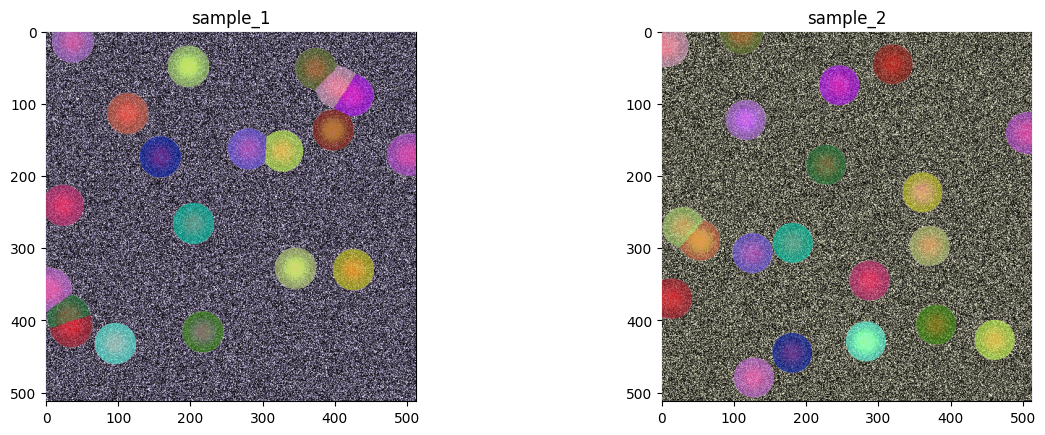
sdata.pl.render_images(channel=selected_markers).pl.render_labels().pl.show(
    coordinate_systems=["sample_1", "sample_2"]
)

harpy.pl.segmentation_size_boxplot(sdata, sample_key="fov_labels")

<Axes: title={'center': 'area'}>

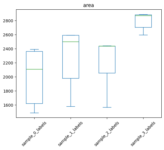
table.obs["area"].describe()

count      80.000000
mean     2349.425000
std       414.222095
min      1489.000000
25%      2069.000000
50%      2437.000000
75%      2593.500000
max      2890.000000
Name: area, dtype: float64

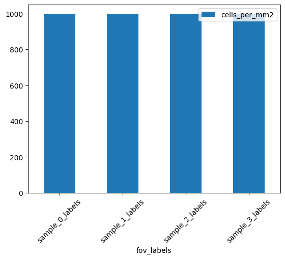
harpy.pl.calculate_segments_per_area(sdata, sample_key="fov_labels")

	fov_labels	cells_per_mm2
fov_labels
sample_0_labels	20	1000
sample_1_labels	20	1000
sample_2_labels	20	1000
sample_3_labels	20	1000

harpy.pl.segments_per_area(sdata, sample_key="fov_labels")

<Axes: xlabel='fov_labels'>

Cell level quality control

import numpy as np

table.layers["arcsinh"] = np.arcsinh(table.to_df())

table

AnnData object with n_obs × n_vars = 80 × 11
    obs: 'instance_id', 'region', 'fov_labels', 'cell_ID', 'phenotype', 'area', 'eccentricity', 'major_axis_length', 'minor_axis_length', 'perimeter', 'centroid-0', 'centroid-1', 'convex_area', 'equivalent_diameter', '_major_minor_axis_ratio', '_perim_square_over_area', '_major_axis_equiv_diam_ratio', '_convex_hull_resid', '_centroid_dif'
    var: 'cycle'
    layers: 'arcsinh'

table.to_df()

	nucleus	lineage_0	lineage_1	lineage_2	lineage_3	lineage_4	lineage_5	lineage_6	lineage_7	lineage_8	lineage_9
cells
1	130579.074583	73143.384718	90176.329291	78887.342227	83547.398858	0.000000	85104.954042	89203.618952	71052.452962	166453.784109	79783.723973
2	97747.257070	44127.352051	54403.315415	47592.677537	50404.086393	0.000000	51343.758329	103611.315408	42865.894408	48557.293269	48133.464008
3	129783.693347	72871.920340	89159.713324	77997.994298	82605.515103	0.000000	132335.765591	88197.968976	70251.432797	79581.243727	78884.270554
4	126967.536598	69764.494608	86010.594981	159287.142678	79687.890840	0.000000	81180.370216	85082.819414	67770.154343	76768.146443	76776.118424
5	107214.353348	52460.254002	64676.705321	56579.963133	124573.992918	0.000000	61039.388909	63979.053282	50960.585762	57726.734557	57222.870407
...	...	...	...	...	...	...	...	...	...	...	...
16	161696.495625	84635.637309	175638.724282	105850.500384	102504.128585	88371.831230	106509.552476	97690.881838	97966.012854	96128.415489	0.000000
17	163295.271990	86338.942986	93873.258186	107784.066049	104567.040494	90150.328405	108653.074179	188483.571632	99937.594462	98063.015157	0.000000
18	153201.459416	75869.389265	82490.085245	94714.053483	91887.127930	80816.560758	95477.684746	87572.419579	175560.397181	86171.787748	0.000000
19	154421.629069	153238.714827	83799.306745	96217.284748	93345.492327	80475.900902	96993.035800	88962.304123	89212.852472	88883.535945	0.000000
20	161275.579840	84186.643485	175348.640010	105097.641133	101960.342041	87903.016819	105944.517075	97172.629669	97446.301109	95618.452236	0.000000

80 rows × 11 columns

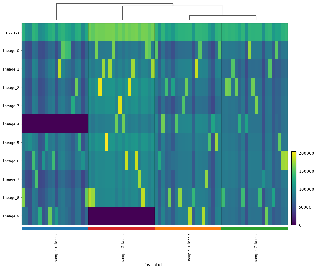
sc.tl.dendrogram(table, groupby="fov_labels")
sc.pl.heatmap(
    table,
    groupby="fov_labels",
    # var_names=used_var_names,
    var_names=table.var_names,
    swap_axes=True,
    dendrogram=True,
    figsize=(12, 10),
)

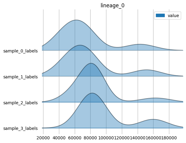
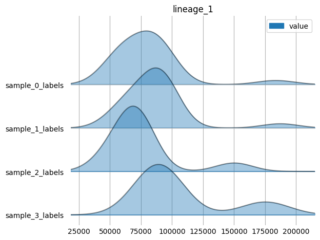
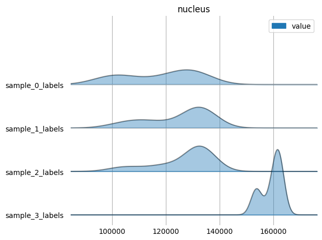
harpy.pl.ridgeplot_channel_sample(table, y="fov_labels", value_vars=selected_markers)

sc.pp.neighbors(table, n_neighbors=10, random_state=42)

sc.tl.umap(table, random_state=42)

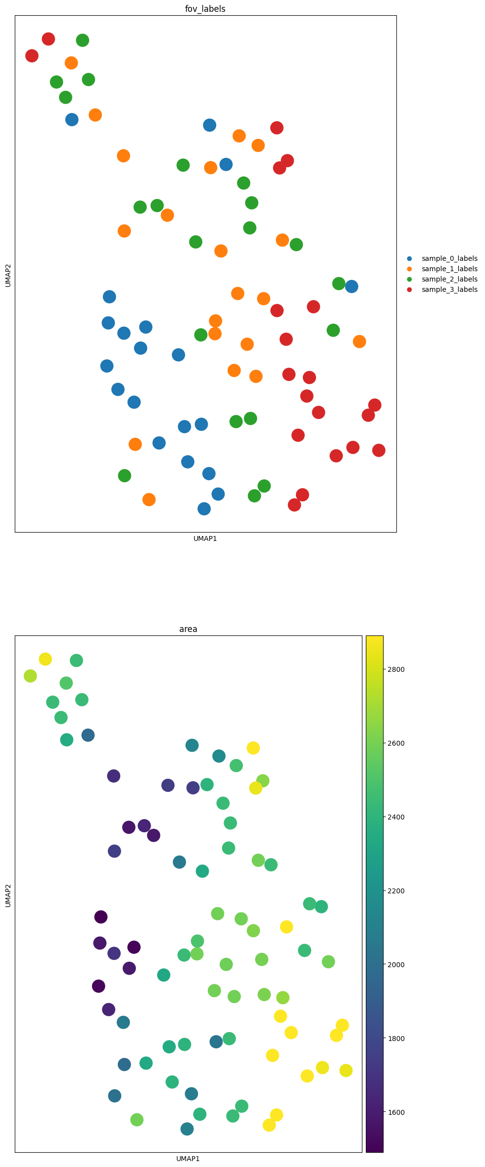
markers = ["fov_labels", "area"]
fig, axes = plt.subplots(len(markers), 1, figsize=(10, 30))
for c, axs in zip(markers, axes, strict=False):
    sc.pl.umap(table, color=c, ax=axs, show=False)

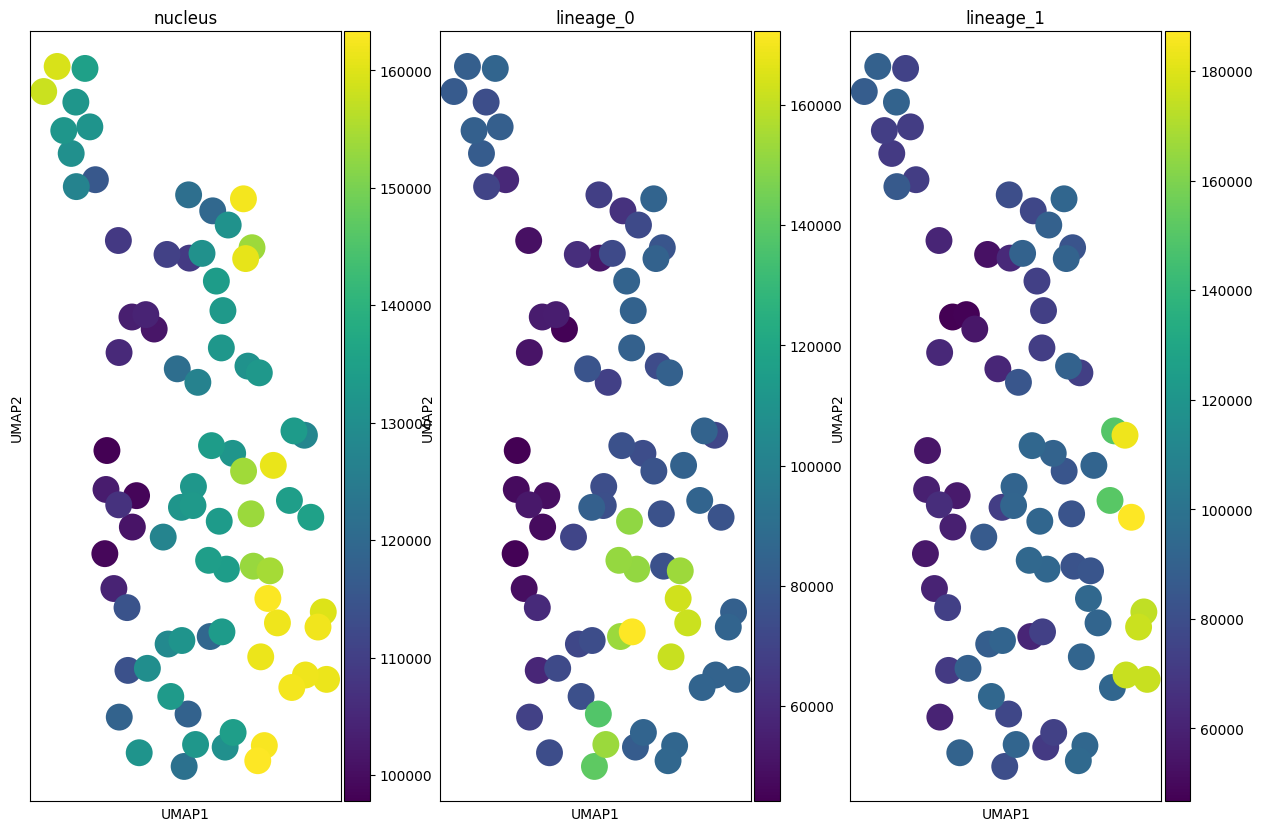
markers = selected_markers
fig, axes = plt.subplots(1, len(markers), figsize=(5 * len(markers), 10))
for c, axs in zip(markers, axes, strict=False):
    sc.pl.umap(table, color=c, ax=axs, show=False)