Quality Control on IMC spatial proteomics with Harpy

Introduction

This noteboook outlines some quality controls steps for highly-multiplexed spatial proteomics data using the Harpy package. Most steps are similar to this good resource on Imaging Mass Cytometry data analysis in R from the Bodenmiller lab. For comparison, the same dataset (IMC data from the Hyperion imaging system) analyzed with steinbock is used in this notebook. The dataset is available in Python as a SpatialData dataset.

The levels of quality control are:

• Image level: to give an overview of the quality of the images in the dataset.

• Segmentation level: to give an overview of the quality of the segmentation in the dataset.

• Cell level: to give an overview of the quality of the calculated features per cell in the dataset.

We start by loading in an example dataset and visualising the data:

import harpy
import matplotlib.pyplot as plt
import scanpy as sc
import spatialdata_plot  # noqa
from harpy.datasets.proteomics import imc_example

plt.viridis()

sdata = imc_example()
sdata

The autoreload extension is already loaded. To reload it, use:
  %reload_ext autoreload

SpatialData object
├── Images
│     ├── 'Patient1_001_image': DataArray[cyx] (40, 600, 600)
│     ├── 'Patient1_002_image': DataArray[cyx] (40, 600, 600)
│     ├── 'Patient1_003_image': DataArray[cyx] (40, 600, 600)
│     ├── 'Patient2_001_image': DataArray[cyx] (40, 600, 600)
│     ├── 'Patient2_002_image': DataArray[cyx] (40, 600, 600)
│     ├── 'Patient2_003_image': DataArray[cyx] (40, 600, 600)
│     ├── 'Patient2_004_image': DataArray[cyx] (40, 600, 600)
│     ├── 'Patient3_001_image': DataArray[cyx] (40, 600, 600)
│     ├── 'Patient3_002_image': DataArray[cyx] (40, 600, 600)
│     ├── 'Patient3_003_image': DataArray[cyx] (40, 600, 600)
│     ├── 'Patient4_005_image': DataArray[cyx] (40, 600, 600)
│     ├── 'Patient4_006_image': DataArray[cyx] (40, 600, 600)
│     ├── 'Patient4_007_image': DataArray[cyx] (40, 600, 600)
│     └── 'Patient4_008_image': DataArray[cyx] (40, 600, 600)
├── Labels
│     ├── 'Patient1_001_labels': DataArray[yx] (600, 600)
│     ├── 'Patient1_002_labels': DataArray[yx] (600, 600)
│     ├── 'Patient1_003_labels': DataArray[yx] (600, 600)
│     ├── 'Patient2_001_labels': DataArray[yx] (600, 600)
│     ├── 'Patient2_002_labels': DataArray[yx] (600, 600)
│     ├── 'Patient2_003_labels': DataArray[yx] (600, 600)
│     ├── 'Patient2_004_labels': DataArray[yx] (600, 600)
│     ├── 'Patient3_001_labels': DataArray[yx] (600, 600)
│     ├── 'Patient3_002_labels': DataArray[yx] (600, 600)
│     ├── 'Patient3_003_labels': DataArray[yx] (600, 600)
│     ├── 'Patient4_005_labels': DataArray[yx] (600, 600)
│     ├── 'Patient4_006_labels': DataArray[yx] (600, 600)
│     ├── 'Patient4_007_labels': DataArray[yx] (600, 600)
│     └── 'Patient4_008_labels': DataArray[yx] (600, 600)
└── Tables
      └── 'table': AnnData (47859, 40)
with coordinate systems:
    ▸ 'Patient1_001', with elements:
        Patient1_001_image (Images), Patient1_001_labels (Labels)
    ▸ 'Patient1_002', with elements:
        Patient1_002_image (Images), Patient1_002_labels (Labels)
    ▸ 'Patient1_003', with elements:
        Patient1_003_image (Images), Patient1_003_labels (Labels)
    ▸ 'Patient2_001', with elements:
        Patient2_001_image (Images), Patient2_001_labels (Labels)
    ▸ 'Patient2_002', with elements:
        Patient2_002_image (Images), Patient2_002_labels (Labels)
    ▸ 'Patient2_003', with elements:
        Patient2_003_image (Images), Patient2_003_labels (Labels)
    ▸ 'Patient2_004', with elements:
        Patient2_004_image (Images), Patient2_004_labels (Labels)
    ▸ 'Patient3_001', with elements:
        Patient3_001_image (Images), Patient3_001_labels (Labels)
    ▸ 'Patient3_002', with elements:
        Patient3_002_image (Images), Patient3_002_labels (Labels)
    ▸ 'Patient3_003', with elements:
        Patient3_003_image (Images), Patient3_003_labels (Labels)
    ▸ 'Patient4_005', with elements:
        Patient4_005_image (Images), Patient4_005_labels (Labels)
    ▸ 'Patient4_006', with elements:
        Patient4_006_image (Images), Patient4_006_labels (Labels)
    ▸ 'Patient4_007', with elements:
        Patient4_007_image (Images), Patient4_007_labels (Labels)
    ▸ 'Patient4_008', with elements:
        Patient4_008_image (Images), Patient4_008_labels (Labels)

<Figure size 640x480 with 0 Axes>

table = sdata["table"]
table

AnnData object with n_obs × n_vars = 47859 × 40
    obs: 'Image', 'area', 'centroid-0', 'centroid-1', 'axis_major_length', 'axis_minor_length', 'eccentricity', 'image', 'image_width_px', 'image_height_px', 'image_num_channels', 'image_source_file', 'image_recovery_file', 'image_recovered', 'image_acquisition_id', 'image_acquisition_description', 'image_acquisition_start_x_um', 'image_acquisition_start_y_um', 'image_acquisition_end_x_um', 'image_acquisition_end_y_um', 'image_acquisition_width_um', 'image_acquisition_height_um', 'cell_id', 'region', 'sample_id', 'patient_id', 'ROI', 'indication'
    var: 'channel', 'name', 'keep', 'ilastik', 'deepcell', 'Tube Number', 'Target', 'Antibody Clone', 'Stock Concentration', 'Final Concentration / Dilution', 'uL to add'
    uns: 'spatialdata_attrs'
    obsm: 'spatial'

table.to_df()

	MPO	HistoneH3	SMA	CD16	CD38	HLADR	CD27	CD15	CD45RA	CD163	...	VISTA	CD40	CD4	CD14	Ecad	CD303	CD206	cleavedPARP	DNA1	DNA2
Object 1 in Patient1_001.tiff	0.575106	3.127308	0.260094	2.034775	0.253014	4.111773	2.307456	7.300499	1.535942	2.166430	...	5.509909	5.162859	7.398499	23.098799	140.415451	9.861239	1.502746	0.672675	75.195312	142.235321
Object 2 in Patient1_001.tiff	0.416667	11.359788	1.672038	2.588054	0.682667	7.646656	1.587182	8.823277	2.303773	6.265749	...	4.544585	5.389460	7.441268	33.736485	65.583473	4.470543	9.239043	0.939726	73.576645	129.302673
Object 3 in Patient1_001.tiff	0.497549	2.384144	0.153519	2.294307	1.190298	13.193821	2.657502	5.005493	1.638779	8.174764	...	4.400037	5.853950	7.854741	26.709986	106.939453	6.576359	4.165048	1.148231	71.255905	119.832062
Object 4 in Patient1_001.tiff	0.890154	7.712961	1.193948	15.629084	2.126060	138.590393	6.149451	5.903136	2.424042	19.541658	...	4.765517	15.262775	24.683125	81.283867	96.895164	7.853501	6.633181	1.260584	59.181263	99.848030
Object 5 in Patient1_001.tiff	0.181818	1.451272	0.298670	0.608422	0.291779	5.911579	0.958761	8.756398	1.549757	0.529756	...	2.797691	1.359595	4.253781	8.609590	74.317711	4.970934	1.286630	0.512645	10.164272	12.806628
...	...	...	...	...	...	...	...	...	...	...	...	...	...	...	...	...	...	...	...	...	...
Object 2841 in Patient4_008.tiff	0.127660	7.424975	0.473410	0.160480	0.230139	0.281806	0.189742	1.311998	0.682346	0.183106	...	0.547729	0.195831	1.727591	3.871677	25.318060	1.705843	0.298129	0.258668	103.932419	180.427872
Object 2842 in Patient4_008.tiff	0.117647	8.225169	0.339634	0.280664	0.374028	0.180113	0.557850	1.664211	0.889153	0.000000	...	0.495479	0.305937	1.954891	5.834383	32.321331	1.414846	0.499866	0.118527	105.321434	187.471375
Object 2843 in Patient4_008.tiff	0.146341	4.159492	0.390537	0.325213	0.340863	0.524208	0.496114	1.371000	0.791754	0.094179	...	0.305323	0.074817	1.589985	4.659936	33.211224	1.783822	0.370879	0.313851	88.465622	164.969193
Object 2844 in Patient4_008.tiff	0.167724	2.898857	0.334794	0.620313	0.083333	0.536346	0.639925	13.249680	0.893656	0.114361	...	0.459324	0.282099	1.955293	6.207744	28.697414	1.973373	0.534088	0.325632	28.828003	50.687141
Object 2845 in Patient4_008.tiff	0.213438	3.275088	0.259993	0.273648	0.094500	0.419652	0.666213	0.861737	0.667140	0.053631	...	0.359852	0.340135	2.530452	8.510514	22.324598	2.136185	0.507724	0.215658	43.971691	73.308266

47859 rows × 40 columns

table.obs

	Image	area	centroid-0	centroid-1	axis_major_length	axis_minor_length	eccentricity	image	image_width_px	image_height_px	...	image_acquisition_end_x_um	image_acquisition_end_y_um	image_acquisition_width_um	image_acquisition_height_um	cell_id	region	sample_id	patient_id	ROI	indication
Object 1 in Patient1_001.tiff	Patient1_001.tiff	12	0.416667	468.583333	7.406234	1.895294	0.966702	Patient1_001.tiff	600	600	...	38100.828	17156.254	600.0	600.0	1	Patient1_001_labels	Patient1_001	Patient1	001	SCCHN
Object 2 in Patient1_001.tiff	Patient1_001.tiff	24	0.416667	515.833333	16.480040	1.962838	0.992882	Patient1_001.tiff	600	600	...	38100.828	17156.254	600.0	600.0	2	Patient1_001_labels	Patient1_001	Patient1	001	SCCHN
Object 3 in Patient1_001.tiff	Patient1_001.tiff	17	0.470588	587.235294	9.850849	1.985817	0.979470	Patient1_001.tiff	600	600	...	38100.828	17156.254	600.0	600.0	3	Patient1_001_labels	Patient1_001	Patient1	001	SCCHN
Object 4 in Patient1_001.tiff	Patient1_001.tiff	24	1.250000	192.250000	8.082904	3.915780	0.874818	Patient1_001.tiff	600	600	...	38100.828	17156.254	600.0	600.0	4	Patient1_001_labels	Patient1_001	Patient1	001	SCCHN
Object 5 in Patient1_001.tiff	Patient1_001.tiff	22	0.909091	231.772727	8.793666	3.116532	0.935091	Patient1_001.tiff	600	600	...	38100.828	17156.254	600.0	600.0	5	Patient1_001_labels	Patient1_001	Patient1	001	SCCHN
...	...	...	...	...	...	...	...	...	...	...	...	...	...	...	...	...	...	...	...	...	...
Object 2841 in Patient4_008.tiff	Patient4_008.tiff	47	597.255319	357.680851	12.607573	5.160594	0.912389	Patient4_008.tiff	600	600	...	28302.627	6595.411	600.0	600.0	2841	Patient4_008_labels	Patient4_008	Patient4	008	CRC
Object 2842 in Patient4_008.tiff	Patient4_008.tiff	17	597.764706	367.058824	5.415619	3.980897	0.677984	Patient4_008.tiff	600	600	...	28302.627	6595.411	600.0	600.0	2842	Patient4_008_labels	Patient4_008	Patient4	008	CRC
Object 2843 in Patient4_008.tiff	Patient4_008.tiff	41	597.731707	136.341463	13.102653	4.112542	0.949466	Patient4_008.tiff	600	600	...	28302.627	6595.411	600.0	600.0	2843	Patient4_008_labels	Patient4_008	Patient4	008	CRC
Object 2844 in Patient4_008.tiff	Patient4_008.tiff	24	597.833333	232.291667	7.790156	4.103809	0.849993	Patient4_008.tiff	600	600	...	28302.627	6595.411	600.0	600.0	2844	Patient4_008_labels	Patient4_008	Patient4	008	CRC
Object 2845 in Patient4_008.tiff	Patient4_008.tiff	30	597.666667	338.666667	9.220415	4.253829	0.887219	Patient4_008.tiff	600	600	...	28302.627	6595.411	600.0	600.0	2845	Patient4_008_labels	Patient4_008	Patient4	008	CRC

47859 rows × 28 columns

selected_markers = ["MPO", "HistoneH3", "SMA"]
sdata.pl.render_images(channel=selected_markers).pl.render_labels().pl.show()

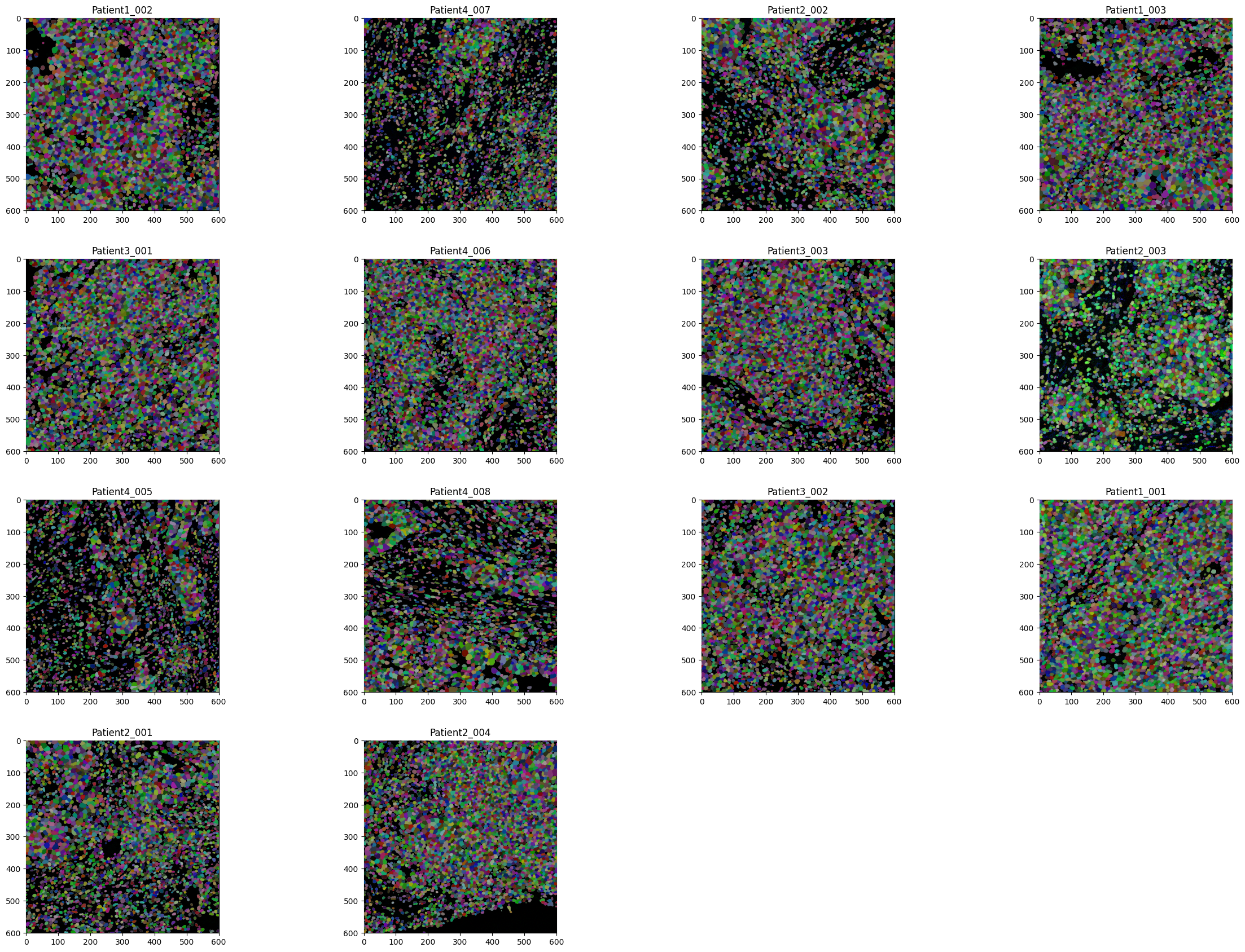
Image level quality control

df = harpy.pl.calculate_snr_ratio(sdata)
df

	image	cycle	channel	snr	signal
0	Patient1_001_image	None	MPO	547.535156	1.241055
1	Patient1_001_image	None	HistoneH3	5.745501	7.948751
2	Patient1_001_image	None	SMA	13.119742	2.827469
3	Patient1_001_image	None	CD16	12.360662	8.994999
4	Patient1_001_image	None	CD38	13.662168	5.337214
...	...	...	...	...	...
555	Patient4_008_image	None	CD303	9.104072	3.356459
556	Patient4_008_image	None	CD206	36.433674	14.416249
557	Patient4_008_image	None	cleavedPARP	1098.977173	1.388665
558	Patient4_008_image	None	DNA1	6.867725	168.084061
559	Patient4_008_image	None	DNA2	6.872324	296.049530

560 rows × 5 columns

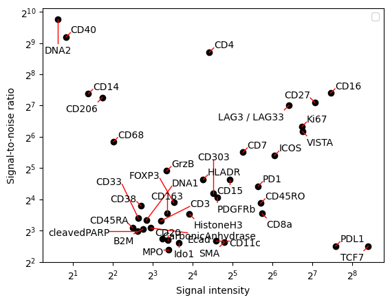
harpy.pl.snr_ratio(sdata)

<Axes: xlabel='Signal intensity', ylabel='Signal-to-noise ratio'>

harpy.pl.snr_ratio(sdata, signal_threshold=2)

<Axes: xlabel='Signal intensity', ylabel='Signal-to-noise ratio'>

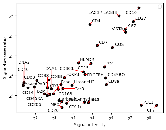
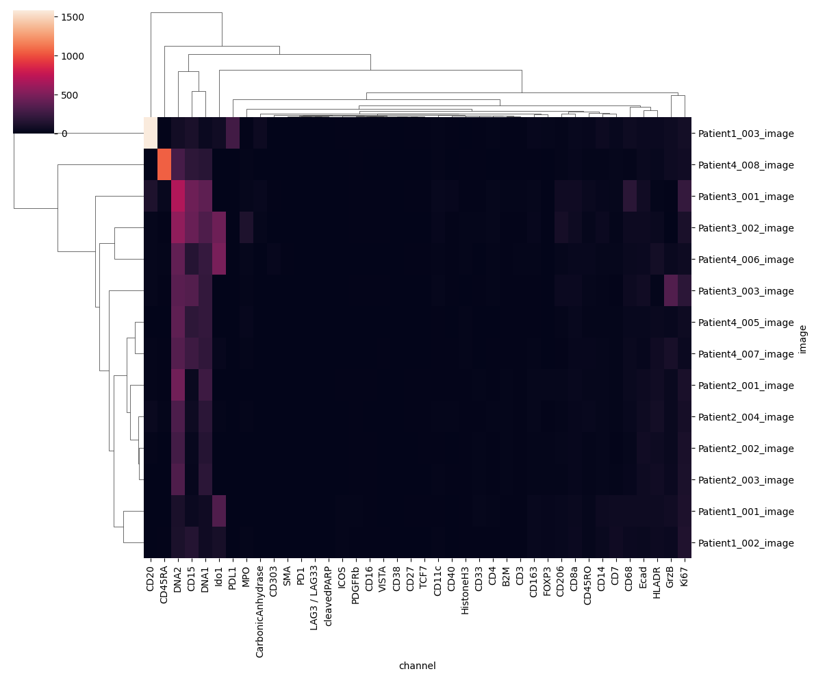
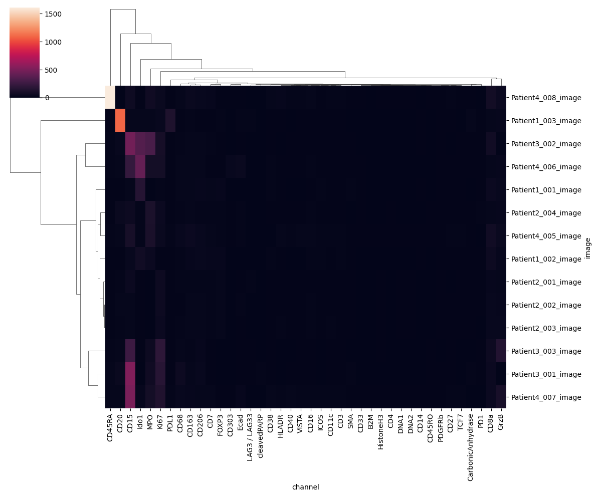
The plots above summarize all samples together. It would be interesting to look without cell segmentation bias across all channels and samples. There are multiple ways to aggregate the channel signal on an image level to a heatmap. One way is to create heatmaps using the SNR and signal values calculated above. This again depends on the unsupervised Otsu thresholding and is not a very good proxy of a good cell segmentation.

When showing the heatmap you could use the z_score or standard_scale options, but it’s also interesting not to transform the data too much in order to still visualize the outliers.

harpy.pl.signal_clustermap(sdata, signal_threshold=2, figsize=(12, 10))

<seaborn.matrix.ClusterGrid at 0x377fc6c80>

harpy.pl.snr_clustermap(sdata, signal_threshold=2, figsize=(12, 10))

<seaborn.matrix.ClusterGrid at 0x36d5080a0>

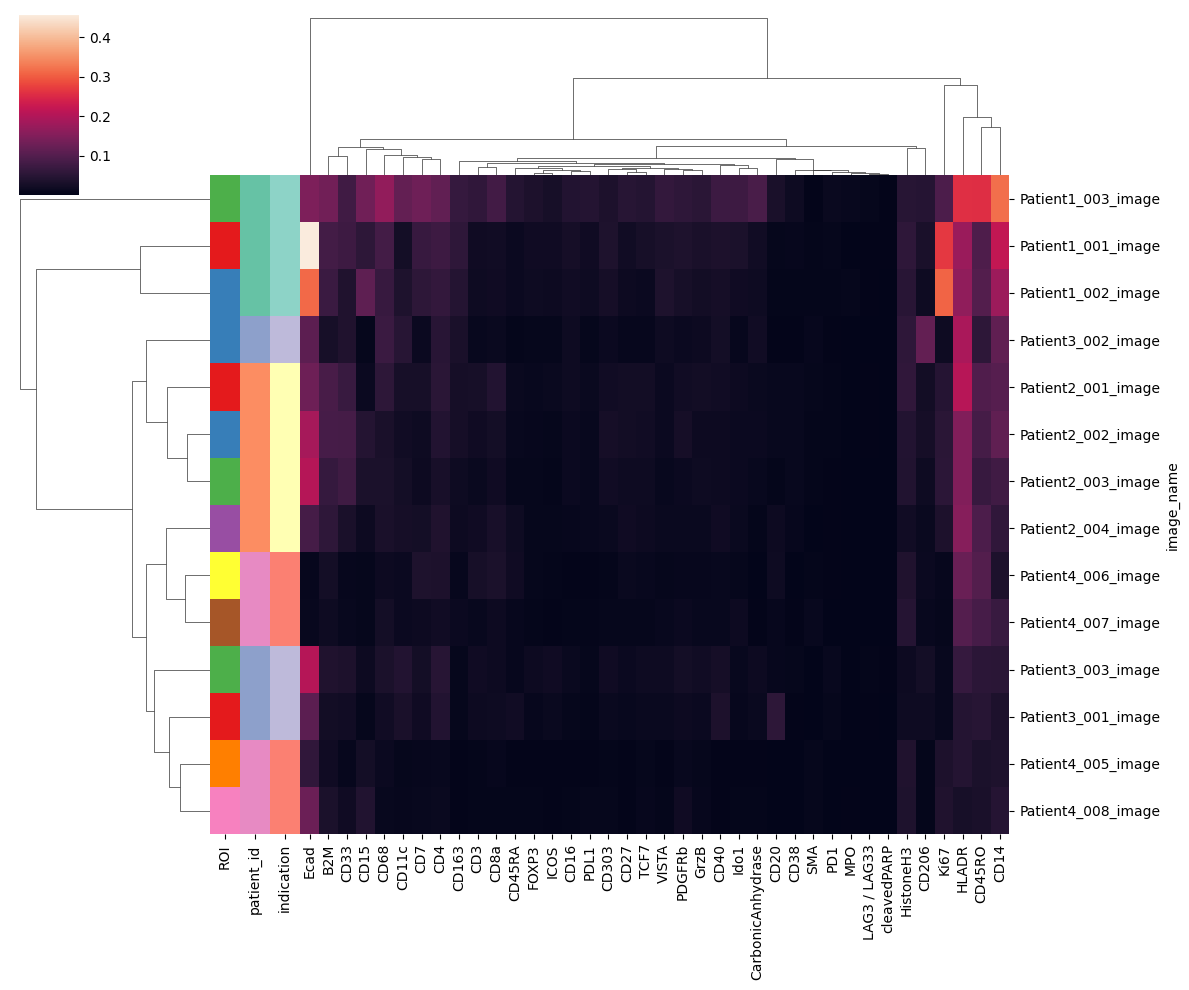
Another way is to normalize the image with a quartile normalization. The min and max quartile can greatly influence how the ends of the intensity distributions. Here we clip the signal below and above the 5th and 95th percentile. We also apply an arcsinh transformation to each channel against extreme outliers to make the heatmap more interpretable.

df_norm = harpy.pl.calculate_mean_norm(
    sdata, overwrite=True, q_min=5, q_max=95, c_mask=["DNA1", "DNA2"]
)
df_norm

	MPO	HistoneH3	SMA	CD16	CD38	HLADR	CD27	CD15	CD45RA	CD163	...	CD33	Ki67	VISTA	CD40	CD4	CD14	Ecad	CD303	CD206	cleavedPARP
image_name
Patient1_001_image	0.001373	0.055785	0.005045	0.026264	0.008826	0.175229	0.020593	0.054659	0.013744	0.056766	...	0.074157	0.267642	0.032680	0.034993	0.074261	0.218794	0.456826	0.036260	0.032173	0.003076
Patient1_002_image	0.006060	0.049233	0.004587	0.020164	0.005141	0.165615	0.015160	0.111997	0.013541	0.043220	...	0.037956	0.307081	0.037028	0.025349	0.062264	0.176832	0.312511	0.025535	0.018039	0.001985
Patient1_003_image	0.010610	0.047956	0.003759	0.042909	0.017612	0.257181	0.047959	0.131205	0.043712	0.066042	...	0.078412	0.092601	0.061601	0.071824	0.114782	0.317894	0.144735	0.034393	0.046012	0.002193
Patient2_001_image	0.000752	0.058385	0.006775	0.016455	0.010782	0.205677	0.022859	0.013033	0.011812	0.026477	...	0.068141	0.045461	0.014171	0.020201	0.050557	0.102343	0.127614	0.020617	0.021694	0.001510
Patient2_002_image	0.000641	0.041701	0.005403	0.013765	0.009545	0.148287	0.022571	0.044532	0.009762	0.026233	...	0.083496	0.051572	0.013299	0.015754	0.041932	0.113859	0.188180	0.026002	0.025739	0.001604
Patient2_003_image	0.000477	0.040524	0.004184	0.014256	0.009770	0.149964	0.016900	0.032347	0.006899	0.016842	...	0.075266	0.052448	0.010327	0.015825	0.029393	0.077996	0.205089	0.021494	0.016302	0.001290
Patient2_004_image	0.000430	0.020642	0.001822	0.007410	0.007910	0.154417	0.018306	0.014674	0.016942	0.014809	...	0.031859	0.035523	0.010955	0.019163	0.038357	0.058413	0.082950	0.011072	0.012548	0.000811
Patient3_001_image	0.000831	0.016921	0.001898	0.006824	0.002759	0.043634	0.009610	0.005878	0.020288	0.006521	...	0.021315	0.009402	0.010975	0.035498	0.041559	0.035015	0.108840	0.012112	0.017181	0.001813
Patient3_002_image	0.001961	0.055722	0.007662	0.017035	0.003206	0.191106	0.008463	0.007178	0.004085	0.032297	...	0.039019	0.017989	0.017073	0.024589	0.048552	0.113121	0.109767	0.013799	0.116642	0.001494
Patient3_003_image	0.001900	0.015013	0.001557	0.010953	0.006222	0.065199	0.014200	0.016212	0.008011	0.006861	...	0.034591	0.009602	0.017635	0.026982	0.047254	0.051440	0.205255	0.019356	0.024959	0.002253
Patient4_005_image	0.001648	0.038940	0.007374	0.002212	0.001156	0.044527	0.003054	0.023514	0.002895	0.003408	...	0.007986	0.035216	0.002902	0.002356	0.009998	0.036888	0.058972	0.005537	0.005516	0.000484
Patient4_006_image	0.000639	0.037834	0.005459	0.002180	0.001767	0.123937	0.011612	0.006143	0.018318	0.008780	...	0.007986	0.008681	0.006178	0.010628	0.035626	0.034305	0.008730	0.004045	0.013496	0.000243
Patient4_007_image	0.000936	0.045258	0.009955	0.004031	0.003228	0.100138	0.006063	0.006296	0.007925	0.014336	...	0.010433	0.007212	0.009297	0.009211	0.020034	0.069162	0.010025	0.007196	0.010052	0.000590
Patient4_008_image	0.002200	0.037542	0.006024	0.004075	0.001709	0.027580	0.003400	0.040889	0.004455	0.003270	...	0.018520	0.039438	0.004279	0.003409	0.012010	0.046535	0.126114	0.007212	0.004356	0.000545

14 rows × 38 columns

df_metadata = table.obs.groupby("sample_id").first()[
    ["ROI", "patient_id", "indication"]
]
df_metadata["image_name"] = df_metadata.index.astype(str) + "_image"
df_metadata.reset_index(inplace=True)
df_metadata.set_index("image_name", inplace=True)
df_metadata.drop("sample_id", axis=1, inplace=True)
df_metadata

	ROI	patient_id	indication
image_name
Patient1_001_image	001	Patient1	SCCHN
Patient1_002_image	002	Patient1	SCCHN
Patient1_003_image	003	Patient1	SCCHN
Patient2_001_image	001	Patient2	BCC
Patient2_002_image	002	Patient2	BCC
Patient2_003_image	003	Patient2	BCC
Patient2_004_image	004	Patient2	BCC
Patient3_001_image	001	Patient3	NSCLC
Patient3_002_image	002	Patient3	NSCLC
Patient3_003_image	003	Patient3	NSCLC
Patient4_005_image	005	Patient4	CRC
Patient4_006_image	006	Patient4	CRC
Patient4_007_image	007	Patient4	CRC
Patient4_008_image	008	Patient4	CRC

harpy.pl.clustermap(
    df_norm, row_colors=harpy.pl.make_cols_colors(df_metadata), figsize=(12, 10)
)

<seaborn.matrix.ClusterGrid at 0x3693fc9a0>

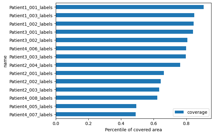
Segmentation level quality control

harpy.pl.segmentation_coverage(sdata)

<Axes: xlabel='Percentile of covered area', ylabel='name'>

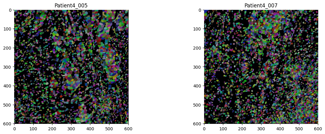
sdata.pl.render_images(channel=selected_markers).pl.render_labels().pl.show(
    coordinate_systems=["Patient4_005", "Patient4_007"]
)

harpy.pl.segmentation_size_boxplot(sdata)

<Axes: title={'center': 'area'}>

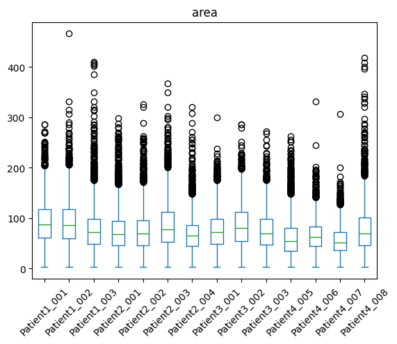
table.obs["area"].describe()

count    47859.000000
mean        76.377296
std         41.443170
min          3.000000
25%         47.000000
50%         70.000000
75%         98.000000
max        466.000000
Name: area, dtype: float64

sum(table.obs["area"] < 5)

65

table[table.obs["area"] >= 5]

View of AnnData object with n_obs × n_vars = 47794 × 40
    obs: 'Image', 'area', 'centroid-0', 'centroid-1', 'axis_major_length', 'axis_minor_length', 'eccentricity', 'image', 'image_width_px', 'image_height_px', 'image_num_channels', 'image_source_file', 'image_recovery_file', 'image_recovered', 'image_acquisition_id', 'image_acquisition_description', 'image_acquisition_start_x_um', 'image_acquisition_start_y_um', 'image_acquisition_end_x_um', 'image_acquisition_end_y_um', 'image_acquisition_width_um', 'image_acquisition_height_um', 'cell_id', 'region', 'sample_id', 'patient_id', 'ROI', 'indication'
    var: 'channel', 'name', 'keep', 'ilastik', 'deepcell', 'Tube Number', 'Target', 'Antibody Clone', 'Stock Concentration', 'Final Concentration / Dilution', 'uL to add'
    uns: 'spatialdata_attrs'
    obsm: 'spatial'

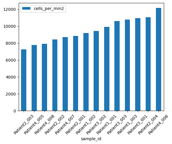
harpy.pl.calculate_segments_per_area(sdata)

	sample_id	image_width_px	image_height_px	cells_per_mm2
sample_id
Patient2_003	2612	600.0	600.0	7255.555556
Patient4_005	2795	600.0	600.0	7763.888889
Patient4_008	2845	600.0	600.0	7902.777778
Patient2_002	3033	600.0	600.0	8425.0
Patient4_007	3135	600.0	600.0	8708.333333
Patient2_001	3185	600.0	600.0	8847.222222
Patient1_002	3304	600.0	600.0	9177.777778
Patient3_002	3393	600.0	600.0	9425.0
Patient1_001	3567	600.0	600.0	9908.333333
Patient3_003	3816	600.0	600.0	10600.0
Patient1_003	3884	600.0	600.0	10788.888889
Patient3_001	3938	600.0	600.0	10938.888889
Patient2_004	3980	600.0	600.0	11055.555556
Patient4_006	4372	600.0	600.0	12144.444444

harpy.pl.segments_per_area(sdata)

<Axes: xlabel='sample_id'>

Cell level quality control

import numpy as np

table.layers["arcsinh"] = np.arcsinh(table.to_df())

table

AnnData object with n_obs × n_vars = 47859 × 40
    obs: 'Image', 'area', 'centroid-0', 'centroid-1', 'axis_major_length', 'axis_minor_length', 'eccentricity', 'image', 'image_width_px', 'image_height_px', 'image_num_channels', 'image_source_file', 'image_recovery_file', 'image_recovered', 'image_acquisition_id', 'image_acquisition_description', 'image_acquisition_start_x_um', 'image_acquisition_start_y_um', 'image_acquisition_end_x_um', 'image_acquisition_end_y_um', 'image_acquisition_width_um', 'image_acquisition_height_um', 'cell_id', 'region', 'sample_id', 'patient_id', 'ROI', 'indication'
    var: 'channel', 'name', 'keep', 'ilastik', 'deepcell', 'Tube Number', 'Target', 'Antibody Clone', 'Stock Concentration', 'Final Concentration / Dilution', 'uL to add'
    uns: 'spatialdata_attrs'
    obsm: 'spatial'
    layers: 'arcsinh'

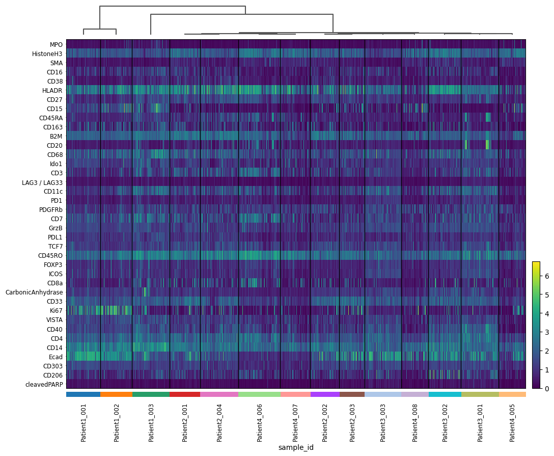
used_var_names = [x for x in table.var_names if x not in ["DNA1", "DNA2"]]
sc.tl.dendrogram(table, groupby="sample_id", var_names=used_var_names)
sc.pl.heatmap(
    table,
    layer="arcsinh",
    groupby="sample_id",
    var_names=used_var_names,
    swap_axes=True,
    dendrogram=True,
    figsize=(12, 10),
)

adata = sc.pp.subsample(table, fraction=0.1, copy=True)
adata

AnnData object with n_obs × n_vars = 4785 × 40
    obs: 'Image', 'area', 'centroid-0', 'centroid-1', 'axis_major_length', 'axis_minor_length', 'eccentricity', 'image', 'image_width_px', 'image_height_px', 'image_num_channels', 'image_source_file', 'image_recovery_file', 'image_recovered', 'image_acquisition_id', 'image_acquisition_description', 'image_acquisition_start_x_um', 'image_acquisition_start_y_um', 'image_acquisition_end_x_um', 'image_acquisition_end_y_um', 'image_acquisition_width_um', 'image_acquisition_height_um', 'cell_id', 'region', 'sample_id', 'patient_id', 'ROI', 'indication'
    var: 'channel', 'name', 'keep', 'ilastik', 'deepcell', 'Tube Number', 'Target', 'Antibody Clone', 'Stock Concentration', 'Final Concentration / Dilution', 'uL to add'
    uns: 'spatialdata_attrs', 'dendrogram_sample_id', 'sample_id_colors'
    obsm: 'spatial'
    layers: 'arcsinh'

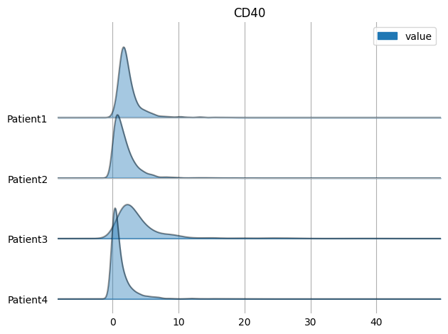
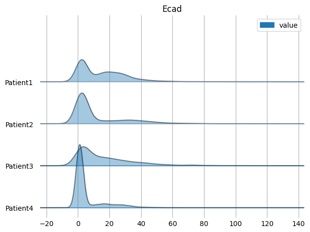
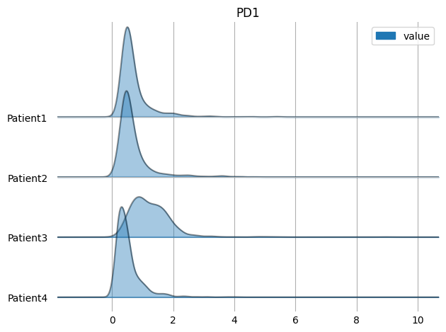
harpy.pl.ridgeplot_channel_sample(
    adata, y="patient_id", value_vars=["Ecad", "CD40", "PD1"]
)

sc.pp.neighbors(table, n_neighbors=10, random_state=42)

sc.tl.umap(table, random_state=42)

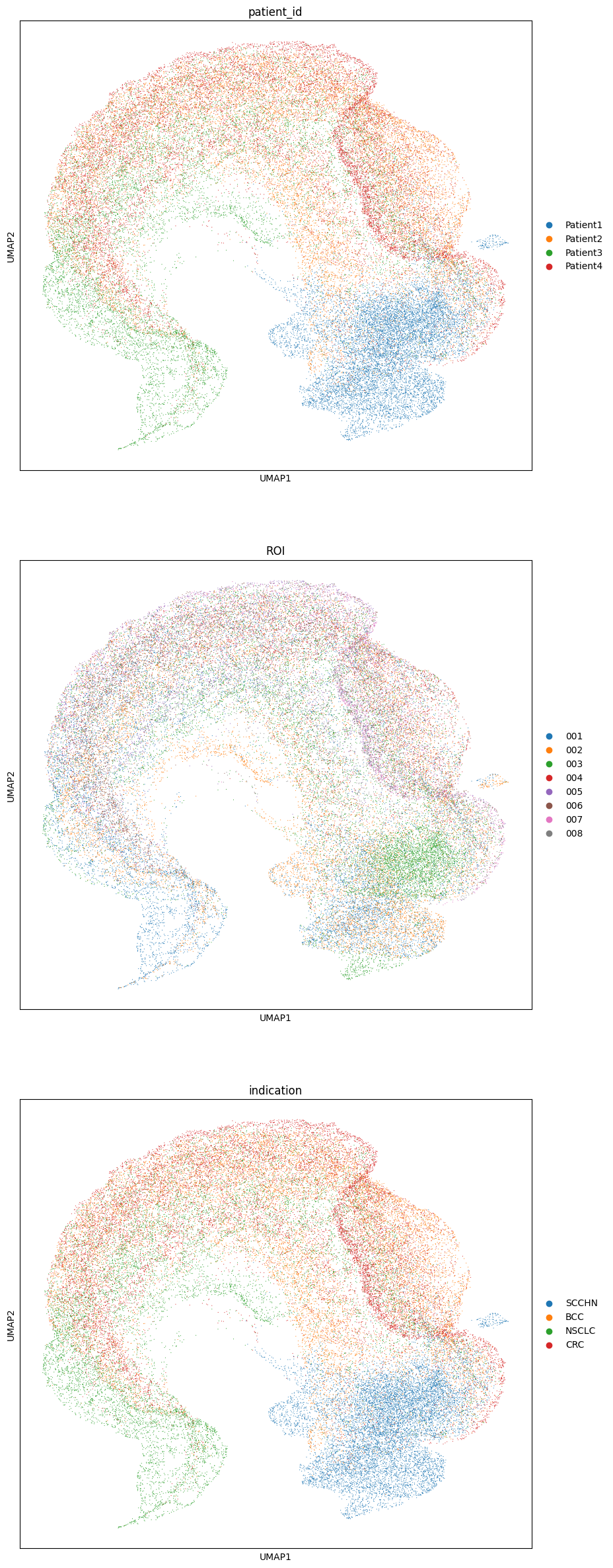
markers = ["patient_id", "ROI", "indication"]
fig, axes = plt.subplots(len(markers), 1, figsize=(10, 30))
for c, axs in zip(markers, axes, strict=False):
    sc.pl.umap(table, color=c, ax=axs, show=False)

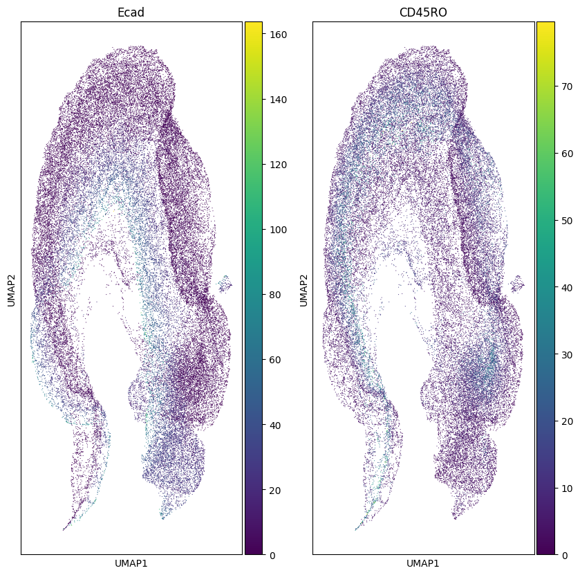
markers = ["Ecad", "CD45RO"]
fig, axes = plt.subplots(1, len(markers), figsize=(5 * len(markers), 10))
for c, axs in zip(markers, axes, strict=False):
    sc.pl.umap(table, color=c, ax=axs, show=False)