Harpy distance calculations#
In this notebook, we perform distance calculations between cells using SpatialData shapes. These shapes may represent regions of interest or simple lines, and can be created through manual annotation in viewers such as napari.
import harpy as hp
import spatialdata as sd
import spatialdata_plot  # noqa
sdata = hp.datasets.cluster_blobs()
sdata
SpatialData object
├── Images
│     └── 'blobs_image': DataArray[cyx] (11, 512, 512)
├── Labels
│     └── 'blobs_labels': DataArray[yx] (512, 512)
├── Points
│     └── 'blobs_points': DataFrame with shape: (<Delayed>, 2) (2D points)
└── Tables
      └── 'table': AnnData (20, 11)
with coordinate systems:
    ▸ 'global', with elements:
        blobs_image (Images), blobs_labels (Labels), blobs_points (Points)
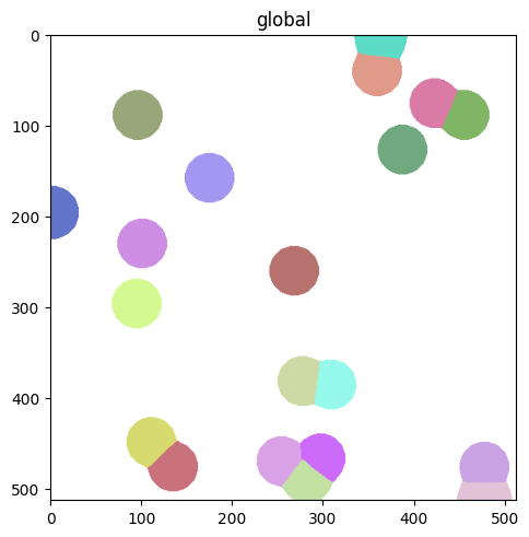
(sdata.pl.render_labels("blobs_labels").pl.show())
# add line and shape to simulate regions
import geopandas as gpd
from shapely.geometry import Polygon, LineString

# note the (x, y) coordinates of the Polygon. In the plotted image it shows x on the bottom and y on the left
roi1 = Polygon([(100, 200), (100, 300), (200, 300), (200, 200)]).buffer(10)
roi2 = Polygon([(300, 400), (300, 500), (400, 500), (400, 400)])
line = LineString([(250, 0), (250, 600)])
roi1

roi_df = gpd.GeoDataFrame(geometry=[roi1, roi2])
line_df = gpd.GeoDataFrame(geometry=[line])
roi_df
| geometry | |
|---|---|
| 0 | POLYGON ((100 190, 99.02 190.048, 98.049 190.1... |
| 1 | POLYGON ((300 400, 300 500, 400 500, 400 400, ... |
roi_df.union_all()

sdata["roi"] = sd.models.ShapesModel.parse(roi_df)
from matplotlib import pyplot as plt

fig, ax = plt.subplots()

(sdata.pl.render_labels("blobs_labels").pl.render_shapes("roi").pl.show(ax=ax))
line_df.plot(ax=ax)
<Axes: title={'center': 'global'}>
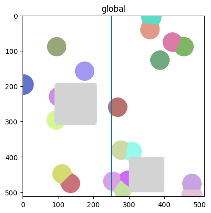
Plotting the Shapes is important to make sure that the coordinates are correct.
Now we want to calculate:
the shortest distance for each cells to any of the two rectangular ROIs.
the shortest distance for each cells to the line.
This is best expressed using Shapely and Geopandas queries. So we will convert the cell labels from the segmentation mask to polygons and then calculate the distances.
To make sure that the distances are calculated correctly, we will plot the ROIs and the line and color the cells according to the distances.
sdata
SpatialData object
├── Images
│     └── 'blobs_image': DataArray[cyx] (11, 512, 512)
├── Labels
│     └── 'blobs_labels': DataArray[yx] (512, 512)
├── Points
│     └── 'blobs_points': DataFrame with shape: (<Delayed>, 2) (2D points)
├── Shapes
│     └── 'roi': GeoDataFrame shape: (2, 1) (2D shapes)
└── Tables
      └── 'table': AnnData (20, 11)
with coordinate systems:
    ▸ 'global', with elements:
        blobs_image (Images), blobs_labels (Labels), blobs_points (Points), roi (Shapes)
cell_polygons = hp.sh.vectorize(
    sdata, labels_name="blobs_labels", output_shapes_name="blobs_shapes", overwrite=True
)  # (sdata["blobs_labels"].data)
cell_polygons["blobs_shapes"]
| geometry | |
|---|---|
| cell_ID | |
| 1 | POLYGON ((249 442, 249 443, 246 443, 246 444, ... |
| 2 | POLYGON ((292 439, 292 440, 289 440, 289 441, ... |
| 3 | POLYGON ((106 421, 106 422, 103 422, 103 423, ... |
| 4 | POLYGON ((170 131, 170 132, 167 132, 167 133, ... |
| 5 | POLYGON ((276 468, 276 470, 275 470, 275 471, ... |
| 6 | POLYGON ((447 62, 447 67, 446 67, 446 70, 445 ... |
| 7 | POLYGON ((453 491, 453 493, 452 493, 452 495, ... |
| 8 | POLYGON ((302 358, 302 359, 297 359, 297 360, ... |
| 9 | POLYGON ((417 49, 417 50, 414 50, 414 51, 411 ... |
| 10 | POLYGON ((0 166, 0 227, 2 227, 2 226, 8 226, 8... |
| 11 | POLYGON ((90 269, 90 270, 87 270, 87 271, 84 2... |
| 12 | POLYGON ((91 62, 91 63, 88 63, 88 64, 85 64, 8... |
| 13 | POLYGON ((382 100, 382 101, 379 101, 379 102, ... |
| 14 | POLYGON ((472 448, 472 449, 469 449, 469 450, ... |
| 15 | POLYGON ((96 203, 96 204, 93 204, 93 205, 90 2... |
| 16 | POLYGON ((338 21, 338 23, 337 23, 337 25, 336 ... |
| 17 | POLYGON ((140 447, 140 448, 138 448, 138 449, ... |
| 18 | POLYGON ((334 0, 334 6, 335 6, 335 12, 336 12,... |
| 19 | POLYGON ((272 354, 272 355, 269 355, 269 356, ... |
| 20 | POLYGON ((263 233, 263 234, 260 234, 260 235, ... |
distances_to_roi = sdata["blobs_shapes"].geometry.distance(roi_df.union_all())
distances_to_roi
cell_ID
1      23.000000
2       0.000000
3     111.000000
4       4.000000
5       0.000000
6     239.771929
7      47.518417
8       0.000000
9     216.417967
10     58.000000
11      0.000000
12     73.000000
13    163.109646
14     50.000000
15      0.000000
16    187.284127
17    137.000000
18    216.024760
19      8.246211
20     31.000000
dtype: float64
from harpy.utils._keys import _INSTANCE_KEY
import numpy as np

# sanity check (check that table matches the created shapes element, so that we are sure that distances are added to correct location)
assert np.array_equal(sdata["table"].obs[_INSTANCE_KEY].values, sdata["blobs_shapes"].index)
sdata["table"].obs["distance_to_roi"] = distances_to_roi.values
sdata["table"].obs["distance_to_line"] = sdata["blobs_shapes"].geometry.distance(line).values
# since SpatialData supports Polygon but not LineString elements, we plot the line separately
fig, ax = plt.subplots()
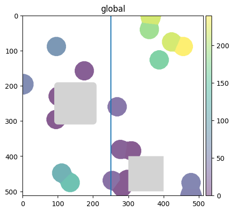
(sdata.pl.render_labels("blobs_labels", color="distance_to_roi").pl.render_shapes("roi").pl.show(ax=ax))
line_df.plot(ax=ax)
<Axes: title={'center': 'global'}>
fig, ax = plt.subplots()

(sdata.pl.render_labels("blobs_labels", color="distance_to_line").pl.render_shapes("roi").pl.show(ax=ax))
line_df.plot(ax=ax)
<Axes: title={'center': 'global'}>
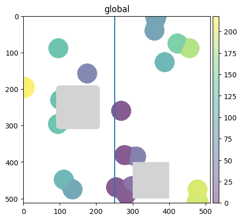
We can see that the cells are colored according to the distance to the line and the two ROIs.
This simple example can be extended to calculate distance to e.g. tumor regions in a tissue. For additional distance analysis or spatial statistics, consider also the documentation of Squidpy or Sopa.