Shallow feature extraction using Harpy.#
Using Harpy, we can compute shallow features for all instances in a labels element based on their corresponding regions in the image element. These features include total intensity, mean intensity, variance, skewness, and more. To do this, we rely on the Harpy function harpy.tb.allocate_intensity (which uses the more general harpy.utils.RasterAggregator).
We also will also illustrate how to calculate more complex statistics using the helper class harpy.utils.Featurizer.
In this notebook, we demonstrate how to extract shallow features from spatial transcriptomics data. The same workflow also applies to spatial proteomics data, see the corresponding notebook.
import harpy as hp
Example 1: Molecular Cartography data.#
from harpy.datasets import resolve_example

sdata = resolve_example()
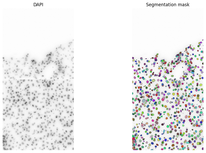
Visualize the segmentation mask.
import matplotlib.pyplot as plt

fig, axes = plt.subplots(1, 2, figsize=(12, 6))  # figsize=(10, 5))

channel = "DAPI"
# normalization parameters for visualization (underlying image not changed)

render_images_kwargs = {"cmap": "binary"}
render_labels_kwargs = {"fill_alpha": 0.6, "outline_alpha": 0.4}
show_kwargs = {
    "title": "DAPI",
    "colorbar": False,
}
_ax = hp.pl.plot_sdata(
    sdata,
    image_name="raw_image",
    channel=0,
    render_images_kwargs=render_images_kwargs,
    show_kwargs=show_kwargs,
    ax=axes[0],
)
_ax.axis("off")

show_kwargs = {
    "title": "Segmentation mask",
    "colorbar": False,
}
_ax = hp.pl.plot_sdata(
    sdata,
    image_name="raw_image",
    labels_name="segmentation_mask",
    channel=0,
    render_images_kwargs=render_images_kwargs,
    render_labels_kwargs=render_labels_kwargs,
    show_kwargs=show_kwargs,
    ax=axes[1],
)
_ax.axis("off")

plt.tight_layout()
plt.show()
INFO     Rasterizing image for faster rendering.
INFO     Rasterizing image for faster rendering.
INFO     Rasterizing image for faster rendering.
Rechunk, so the labels element and image element have same spatial ((‘z’), ‘y’, ‘x’) chunk size.
# first make sure image element and labels element have the same chunk size
chunk_size = 1024
image_name = "raw_image"
labels_name = "segmentation_mask"

# rechunk
sdata = hp.im.add_image(
    sdata,
    arr=hp.im.get_dataarray(sdata, element_name=image_name).data.rechunk(chunk_size),
    output_image_name=image_name,
    c_coords=["DAPI"],
    overwrite=True,
)

sdata = hp.im.add_labels(
    sdata,
    arr=hp.im.get_dataarray(sdata, element_name=labels_name).data.rechunk(chunk_size),
    output_labels_name=labels_name,
    overwrite=True,
)
Now, lets aggregate the image and labels element and calculate the following shallow features: 'sum', ‘var’, ‘skew’, ‘count’(=instance size).
The total intensity ('sum'), will be added to the .X attribute of the AnnData table. The other features will be added to the .obs attribute of the table.
sdata = hp.tb.allocate_intensity(
    sdata,
    image_name="raw_image",
    labels_name="segmentation_mask",
    output_table_name="table_intensities",
    mode="sum",
    obs_stats=["var", "skew", "count"],  # count will be added as "nucleus_size" in .obs
    instance_size_key="nucleus_size",
    calculate_center_of_mass=True,
    spatial_key="spatial",
)

display(sdata["table_intensities"])
display(sdata["table_intensities"].to_df().head())
display(sdata["table_intensities"].obs.head())
display(sdata["table_intensities"].obsm["spatial"][:5])  # -> center of mask
AnnData object with n_obs × n_vars = 657 × 1
    obs: 'cell_ID', 'fov_labels', 'var_DAPI', 'skew_DAPI', 'nucleus_size'
    uns: 'spatialdata_attrs'
    obsm: 'spatial'
| channels | DAPI |
|---|---|
| cells | |
| 1_segmentation_mask_64d9012c | 1675982.0 |
| 2_segmentation_mask_64d9012c | 4928528.0 |
| 4_segmentation_mask_64d9012c | 4872624.0 |
| 5_segmentation_mask_64d9012c | 2925965.0 |
| 7_segmentation_mask_64d9012c | 2936661.0 |
| cell_ID | fov_labels | var_DAPI | skew_DAPI | nucleus_size | |
|---|---|---|---|---|---|
| cells | |||||
| 1_segmentation_mask_64d9012c | 1 | segmentation_mask | 801741.250000 | -0.415835 | 1063.0 |
| 2_segmentation_mask_64d9012c | 2 | segmentation_mask | 293185.375000 | -0.541046 | 2317.0 |
| 4_segmentation_mask_64d9012c | 4 | segmentation_mask | 320540.906250 | -0.103748 | 2192.0 |
| 5_segmentation_mask_64d9012c | 5 | segmentation_mask | 168423.765625 | 0.753061 | 1777.0 |
| 7_segmentation_mask_64d9012c | 7 | segmentation_mask | 461050.093750 | 0.161739 | 1417.0 |
array([[2125.67638758,  961.25117592],
       [2068.32887354, 1036.62926198],
       [2016.3020073 , 1052.68385036],
       [2033.00844119, 1103.77940349],
       [1748.87579393, 1120.17431193]])
# visualize the info with spatialdata-plot

fig, axes = plt.subplots(1, 2, figsize=(12, 6))

# normalization parameters for visualization (underlying image not changed)
se = hp.im.get_dataarray(sdata, element_name="raw_image")

channel = "DAPI"

render_images_kwargs = {"cmap": "binary"}
render_labels_kwargs = {"fill_alpha": 0.6, "outline_alpha": 0.4}

# color by area
color = "nucleus_size"
show_kwargs = {
    "title": "Nucleus size",
    "colorbar": True,
}
ax = hp.pl.plot_sdata(
    sdata,
    image_name="raw_image",
    channel=channel,
    labels_name="segmentation_mask",
    table_name="table_intensities",
    color=color,
    render_images_kwargs=render_images_kwargs,
    show_kwargs=show_kwargs,
    ax=axes[0],
)
ax.axis("off")

# color by mean intensity
color = channel
show_kwargs = {
    "title": f"{color} intensity per nucleus",
    "colorbar": True,
}
ax = hp.pl.plot_sdata(
    sdata,
    image_name="raw_image",
    channel=channel,
    labels_name="segmentation_mask",
    table_name="table_intensities",
    color=color,
    render_images_kwargs=render_images_kwargs,
    show_kwargs=show_kwargs,
    ax=axes[1],
)
ax.axis("off")

plt.tight_layout()
plt.show()
INFO     Rasterizing image for faster rendering.
INFO     Rasterizing image for faster rendering.
INFO     Rasterizing image for faster rendering.
INFO     Rasterizing image for faster rendering.
We also can extract geometric and morphological information based on the shape of the cells and append it as extra observations to our table. This can be useful to distinguish between different cell types. For example, we can calculate the area of the cell, the perimeter, the eccentricity, the solidity, the major and minor axis.
sdata = hp.tb.add_regionprop_features(
    sdata,
    labels_name="segmentation_mask",
    table_name="table_intensities",
    output_table_name="table_intensities",
    properties=["perimeter", "eccentricity"],
    overwrite=True,
)
display(sdata["table_intensities"].obs.head())
| cell_ID | fov_labels | var_DAPI | skew_DAPI | nucleus_size | perimeter | eccentricity | |
|---|---|---|---|---|---|---|---|
| cells | |||||||
| 1_segmentation_mask_64d9012c | 1 | segmentation_mask | 801741.250000 | -0.415835 | 1063.0 | 127.254834 | 0.756004 |
| 2_segmentation_mask_64d9012c | 2 | segmentation_mask | 293185.375000 | -0.541046 | 2317.0 | 180.953319 | 0.491016 |
| 4_segmentation_mask_64d9012c | 4 | segmentation_mask | 320540.906250 | -0.103748 | 2192.0 | 177.781746 | 0.675326 |
| 5_segmentation_mask_64d9012c | 5 | segmentation_mask | 168423.765625 | 0.753061 | 1777.0 | 156.124892 | 0.569551 |
| 7_segmentation_mask_64d9012c | 7 | segmentation_mask | 461050.093750 | 0.161739 | 1417.0 | 157.231493 | 0.795358 |
For computing statistics such as quantiles or principal axes of a segmentation mask, we provide the helper class harpy.utils.Featurizer. This class extracts individual instances from multiplex imaging data and computes statistics for each instance.
For example, quantiles and principal axes of the segmentation mask can be computed as follows:
img_array = sdata[image_name].data[:, None, ...]
mask_array = sdata[labels_name].data[None, ...]

fe = hp.utils.Featurizer(mask_dask_array=mask_array, image_dask_array=img_array)
df_quantiles = fe.quantiles(
    diameter=100,
    depth=50,
    q=[0.1, 0.3, 0.5, 0.7, 0.9],
)
display(df_quantiles[0].head())  # -> 0.1 quantile intensity for each cell and each channel
display(df_quantiles[-1].head())  # -> 0.9 quantile

df_radii = fe.radii_and_principal_axes(
    diameter=100,
    depth=50,
    calculate_axes=False,
)
display(df_radii.head())  # radii
| 0 | cell_ID | |
|---|---|---|
| 0 | 0.000000 | 1 |
| 1 | 1238.000000 | 2 |
| 2 | 1370.500000 | 4 |
| 3 | 1163.199951 | 5 |
| 4 | 1191.000000 | 7 |
| 0 | cell_ID | |
|---|---|---|
| 0 | 2644.000000 | 1 |
| 1 | 2727.000000 | 2 |
| 2 | 2804.899902 | 4 |
| 3 | 2179.000000 | 5 |
| 4 | 3047.000000 | 7 |
| 0 | 1 | 2 | cell_ID | |
|---|---|---|---|---|
| 0 | 11.452508 | 7.496437 | 0.0 | 1 |
| 1 | 14.585308 | 12.705996 | 0.0 | 2 |
| 2 | 15.416794 | 11.370177 | 0.0 | 4 |
| 3 | 13.131853 | 10.793805 | 0.0 | 5 |
| 4 | 13.820557 | 8.377190 | 0.0 | 7 |
A statistic of choice can be calculated using the method hp.utils.Featurizer.calculate_instance_statistics(), we refer to the docstring for an example.
Example 2: Merscope data.#
sdata = hp.datasets.merscope_mouse_liver_segmentation_mask()
Back the data to a Zarr store for optimal processing.
import os

from spatialdata import read_zarr

path = os.environ.get("TMPDIR")  # This path can be changed to any output folder.

sdata.write(os.path.join(path, "sdata_merscope.zarr"), overwrite=True)
sdata = read_zarr(sdata.path)
First make sure the image and labels element have the same chunk size on disk, for optimal processing.
# first make sure image element and labels element have the same chunk size

chunk_size = 4096  # pick a chunksize that is not too small
image_name = "clahe"
labels_name = "segmentation_mask_full"

# rechunk on disk
sdata = hp.im.add_image(
    sdata,
    arr=hp.im.get_dataarray(sdata, element_name=image_name).data.rechunk(chunk_size),
    output_image_name=image_name,
    c_coords=["DAPI", "PolyT"],
    scale_factors=[2, 2, 2, 2],
    overwrite=True,
)

sdata = hp.im.add_labels(
    sdata,
    arr=hp.im.get_dataarray(sdata, element_name=labels_name).data.rechunk(chunk_size),
    output_labels_name=labels_name,
    scale_factors=[2, 2, 2, 2],
    overwrite=True,
)
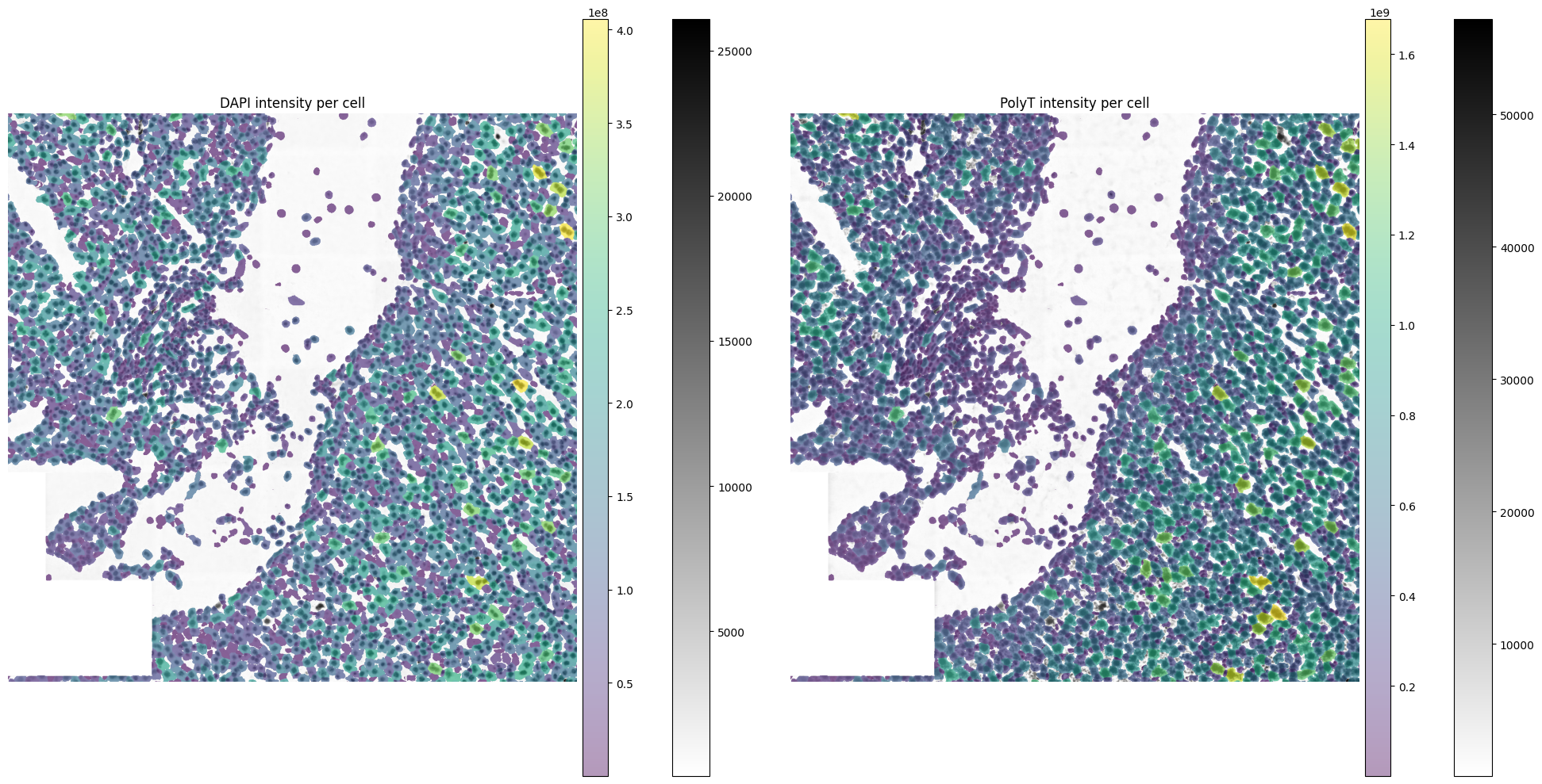
Now calculate the total intensity for every cell, and for every channel using harpy.tb.allocate_intensity.
from dask.distributed import Client, LocalCluster

cluster = LocalCluster(
    n_workers=8,  # using workers instead of threads is slightly faster on large datasets.
    threads_per_worker=1,
    memory_limit="500GB",  # prevent spilling to disk
    local_directory=os.environ.get("SCRATCHDIR"),
)

client = Client(cluster)
print(client.dashboard_link)

sdata = hp.tb.allocate_intensity(
    sdata,
    image_name=image_name,
    labels_name=labels_name,
    output_table_name="table_intensities",
    mode="sum",
    calculate_center_of_mass=False,
    overwrite=True,
)  # takes around 2 minutes

client.close()
display(sdata["table_intensities"].to_df().head())
| channels | DAPI | PolyT |
|---|---|---|
| cells | ||
| 1025_segmentation_mask_full_20d49a42 | 12554694.0 | 50630048.0 |
| 1026_segmentation_mask_full_20d49a42 | 114171.0 | 406149.0 |
| 1027_segmentation_mask_full_20d49a42 | 1000944.0 | 7133834.0 |
| 1028_segmentation_mask_full_20d49a42 | 10002447.0 | 26179680.0 |
| 1031_segmentation_mask_full_20d49a42 | 10884798.0 | 35758056.0 |
import matplotlib.pyplot as plt

fig, axes = plt.subplots(1, 2, figsize=(20, 10))

se = hp.im.get_dataarray(sdata, element_name="clahe")

channels = se.c.data

render_images_kwargs = {"cmap": "binary"}
render_labels_kwargs = {"fill_alpha": 0.6, "outline_alpha": 0.4}

# subset, because query is slow on points element
sdata_to_plot = sdata.subset(element_names=[image_name, labels_name])

for channel, ax in zip(channels, axes, strict=True):
    color = channel
    show_kwargs = {
        "title": f"{color} intensity per cell",
        "colorbar": True,
    }
    ax = hp.pl.plot_sdata(
        sdata_to_plot,
        image_name=image_name,
        channel=channel,
        labels_name=labels_name,
        table_name="table_intensities",
        crd=[20000, 30000, 20000, 30000],
        color=color,
        render_images_kwargs=render_images_kwargs,
        show_kwargs=show_kwargs,
        to_coordinate_system="global",
        ax=ax,
    )
    ax.axis("off")

plt.tight_layout()
plt.show()