Run FlowSOM for pixel and cell clustering#
This notebook provides an implementation of unsupervised pixel and cell level clustering approach described in Liu, C.C., Greenwald, N.F., Kong, A., et al. (2023). Robust phenotyping of highly multiplexed tissue imaging data using pixel-level clustering. Nature Communications, 14, 4618. https://doi.org/10.1038/s41467-023-40068-5.
This implementation follows the methodology of the original ark-analysis repository but has been reengineered for compatibility with SpatialData and leverages Dask for efficient scaling to gigapixel-scale images.
You can run this notebook, without installing squidpy, but to run the cell that calls hp.tb.spatial_pixel_neighbors, you’ll need to install it.
import harpy as hp
from harpy.datasets import pixie_example
from harpy.utils._keys import ClusteringKey

# supress warnings
import warnings

warnings.filterwarnings(
    "ignore", message="The table is annotating", category=UserWarning
)
1. Load example dataset#
import os
import tempfile

from spatialdata import read_zarr

sdata = pixie_example()

# back the spatialdata object to a zarr store:

OUTPUT_DIR = tempfile.gettempdir()

zarr_path = os.path.join(OUTPUT_DIR, "sdata_pixie.zarr")

sdata.write(zarr_path, overwrite=True)
sdata = read_zarr(sdata.path)
channels = [
    "CD3",
    "CD4",
    "CD8",
    "CD14",
    "CD20",
    "CD31",
    "CD45",
    "CD68",
    "CD163",
    "CK17",
    "Collagen1",
    "Fibronectin",
    "ECAD",
    "HLADR",
    "SMA",
    "Vim",
]
import numpy as np
import dask.array as da
from matplotlib.colors import Normalize
import matplotlib.pyplot as plt
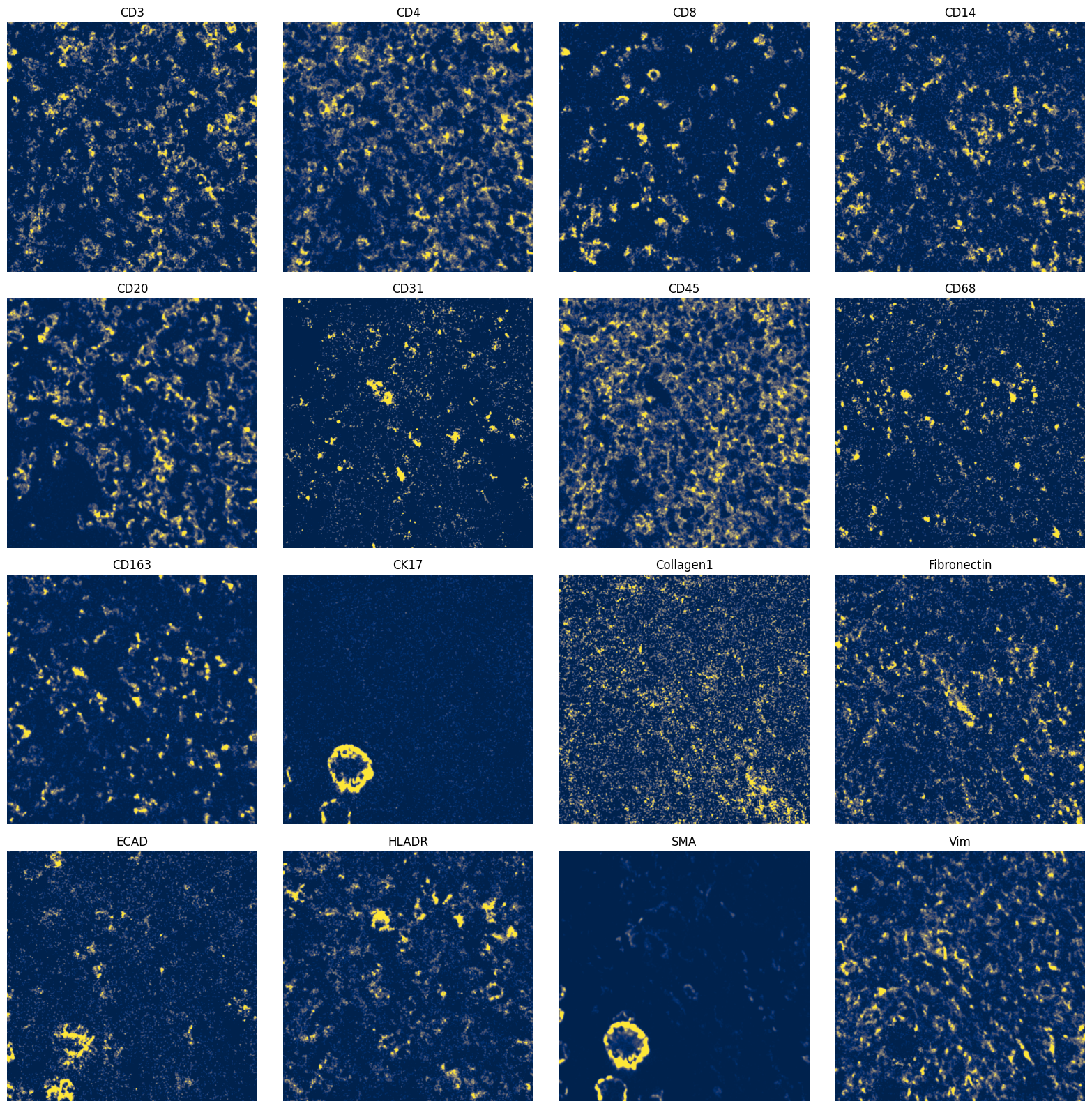
fig, axes = plt.subplots(4, 4, figsize=(16, 16))
_image_name = "raw_image_fov0"
to_coordinate_system = "fov0"
for _ax, _channel in zip(axes.flatten(), channels, strict=True):
# normalization parameters for visualization (underlying image not changed)
se = hp.im.get_dataarray(sdata, element_name=_image_name)
_channel_idx = np.where(sdata[_image_name].c.data == _channel)[0].item()
vmax = da.percentile(se.data[_channel_idx].flatten(), q=99).compute()
norm = Normalize(vmax=vmax, clip=False)
render_images_kwargs = {"cmap": "cividis", "norm": norm}
show_kwargs = {"title": _channel, "colorbar": False}
_ax = hp.pl.plot_sdata(
sdata,
image_name=_image_name,
channel=_channel,
to_coordinate_system=to_coordinate_system,
render_images_kwargs=render_images_kwargs,
show_kwargs=show_kwargs,
ax=_ax,
)
# frameless figure
_ax.axis("off")
plt.tight_layout()
plt.show()
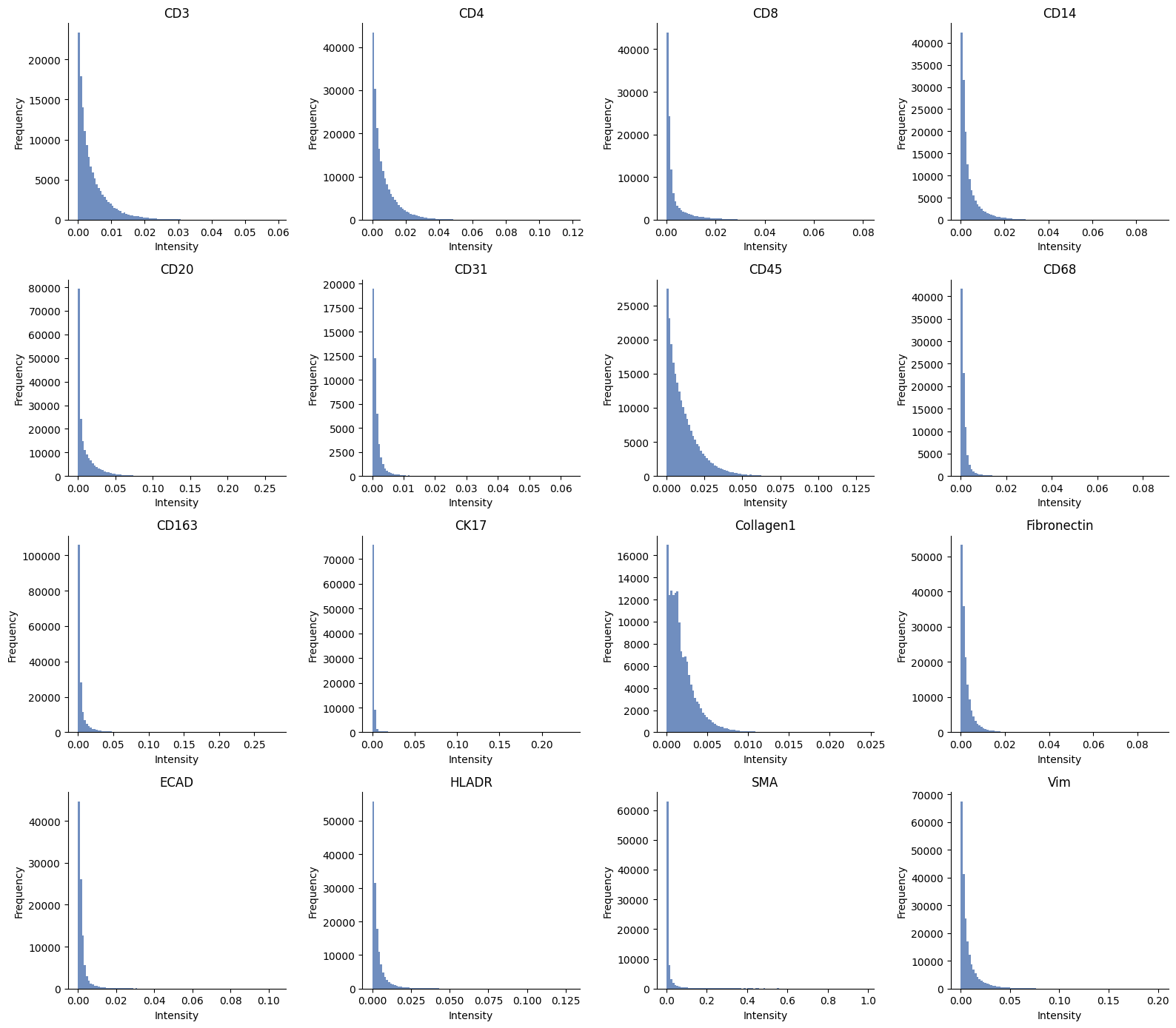
ax = hp.qc.image_histogram(
    sdata,
    image_name="raw_image_fov0",
    channel=channels,
    ncols=4,
    bins=100,
)
2. Preprocess#
N = 11  # set to 11 to process all samples

image_name = [f"raw_image_fov{i}" for i in range(N)]

sdata = hp.im.pixel_clustering_preprocess(
    sdata,
    image_name=image_name,
    output_image_name=[f"{_image_name}_processed" for _image_name in image_name],
    channels=channels,
    chunks=2048,
    persist_intermediate=True,  # set to False if you have multiple images, and if they are large.
    overwrite=True,
    sigma=2.0,
)
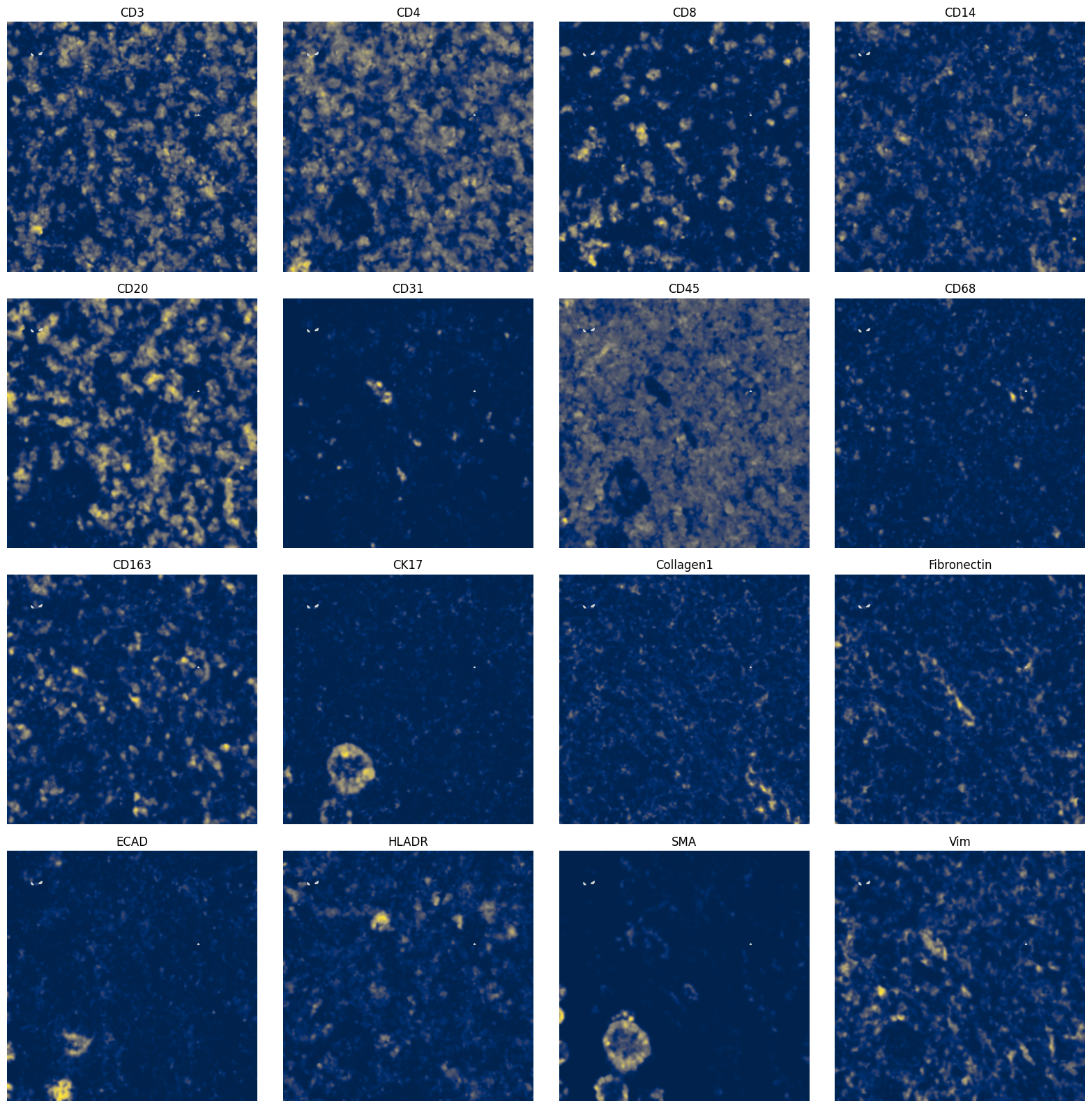
fig, axes = plt.subplots(4, 4, figsize=(16, 16))
_image_name = "raw_image_fov0_processed"
to_coordinate_system = "fov0"

for _ax, _channel in zip(axes.flatten(), channels, strict=True):
    render_images_kwargs = {"cmap": "cividis", "norm": None}
    show_kwargs = {"title": _channel, "colorbar": False}
    _ax = hp.pl.plot_sdata(
        sdata,
        image_name=_image_name,
        channel=_channel,
        to_coordinate_system=to_coordinate_system,
        render_images_kwargs=render_images_kwargs,
        show_kwargs=show_kwargs,
        ax=_ax,
    )
    # frameless figure
    _ax.axis("off")

plt.tight_layout()
plt.show()
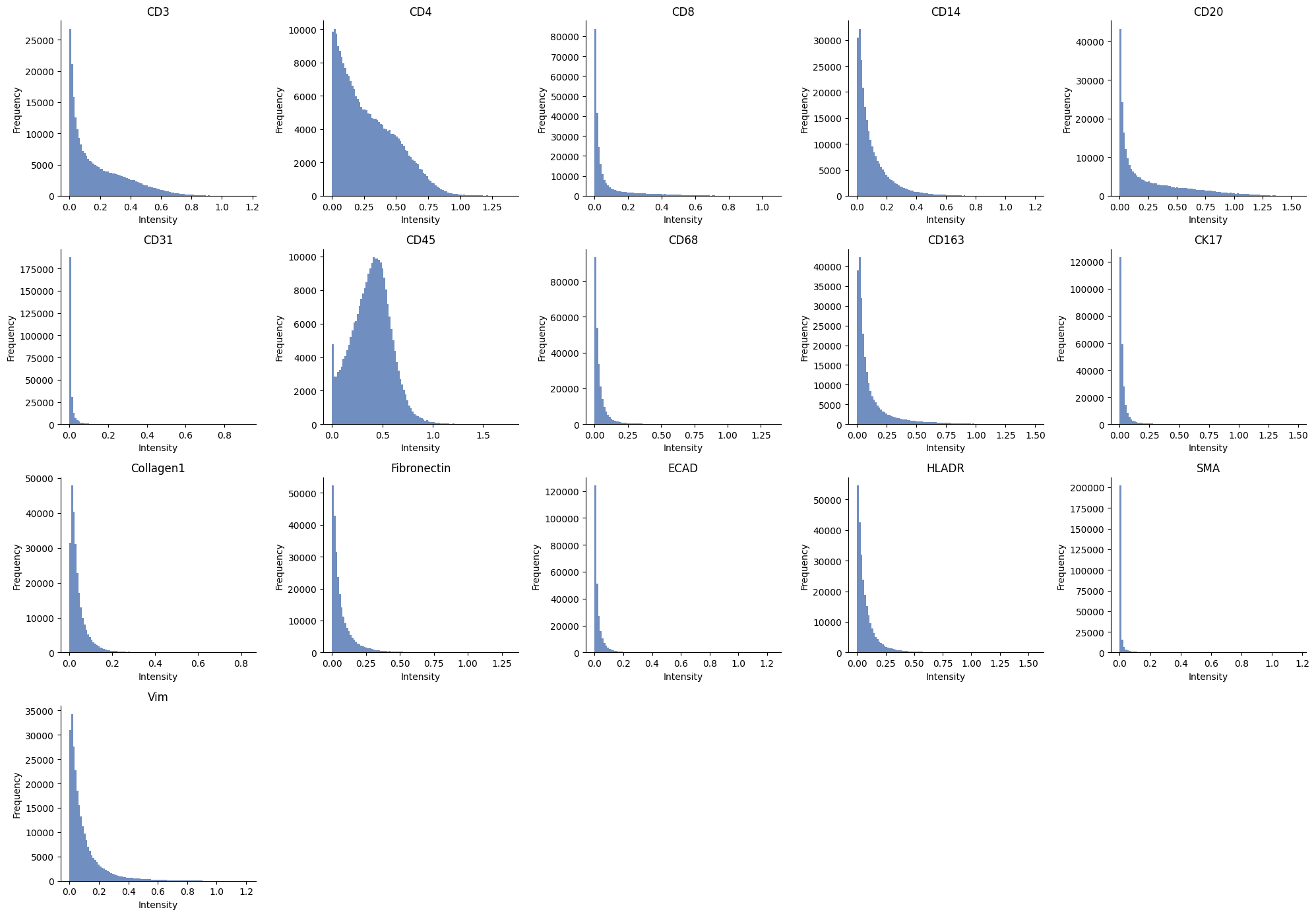
ax = hp.qc.image_histogram(
    sdata,
    image_name="raw_image_fov0_processed",
    channel=channels,
    ncols=5,
    bins=100,
)
3. Pixel clustering#
import flowsom as fs
from dask.distributed import Client, LocalCluster

work_with_client = True

if work_with_client:
    # client example
    cluster = LocalCluster(
        n_workers=1,
        threads_per_worker=10,
    )

    client = Client(cluster)
    print(f"Dashboard link: {client.dashboard_link}")
else:
    client = None

batch_model = fs.models.BatchFlowSOMEstimator

sdata, fsom, mapping = hp.im.flowsom(
    sdata,
    image_name=[f"{_image_name}_processed" for _image_name in image_name],
    output_cluster_labels_name=[
        f"{_image_name}_flowsom_clusters" for _image_name in image_name
    ],  # we need output_cluster_layer and output_meta_cluster_layer --> these will both be labels elements
    output_metacluster_labels_name=[
        f"{_image_name}_flowsom_metaclusters" for _image_name in image_name
    ],
    n_clusters=20,
    random_state=111,
    chunks=512,
    client=client,
    model=batch_model,
    num_batches=10,
    xdim=10,
    ydim=10,
    z_score=True,
    z_cap=3,
    persist_intermediate=True,
    overwrite=True,
)

if client is not None:
    client.close()
Dashboard link: http://127.0.0.1:52588/status
sdata = hp.tb.cluster_intensity_SOM(
    sdata,
    mapping=mapping,
    image_name=[f"{_image_name}_processed" for _image_name in image_name],
    labels_name=[f"{_image_name}_flowsom_clusters" for _image_name in image_name],
    to_coordinate_system=[f"fov{i}" for i in range(N)],
    output_table_name="counts_clusters",
    overwrite=True,
)
4. Visualization of pixel clusters and metaclusters#
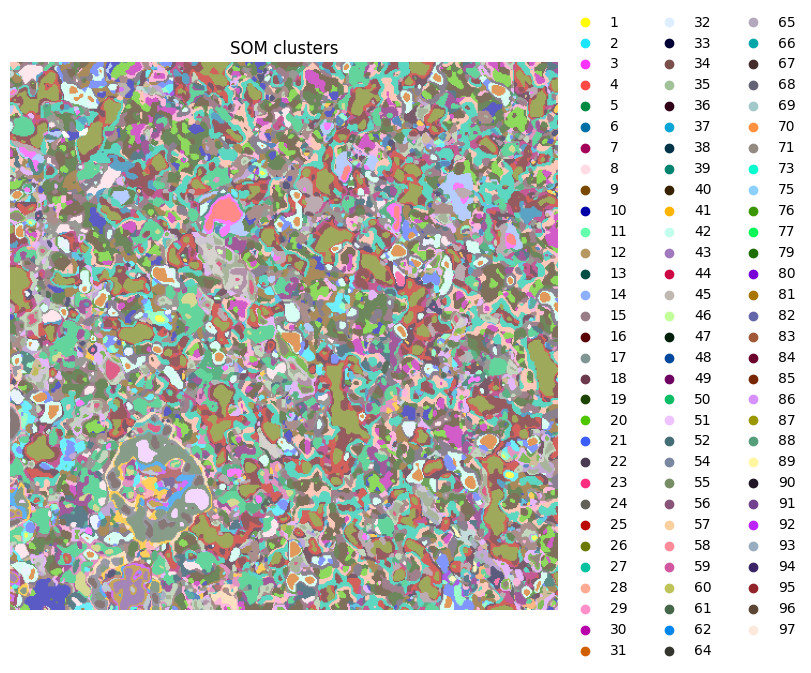
ax = hp.pl.pixel_clusters(
sdata,
labels_name="raw_image_fov0_flowsom_clusters",
figsize=(8, 8),
to_coordinate_system="fov0",
render_labels_kwargs={"alpha": 1},
title="SOM clusters",
)
ax.axis("off")
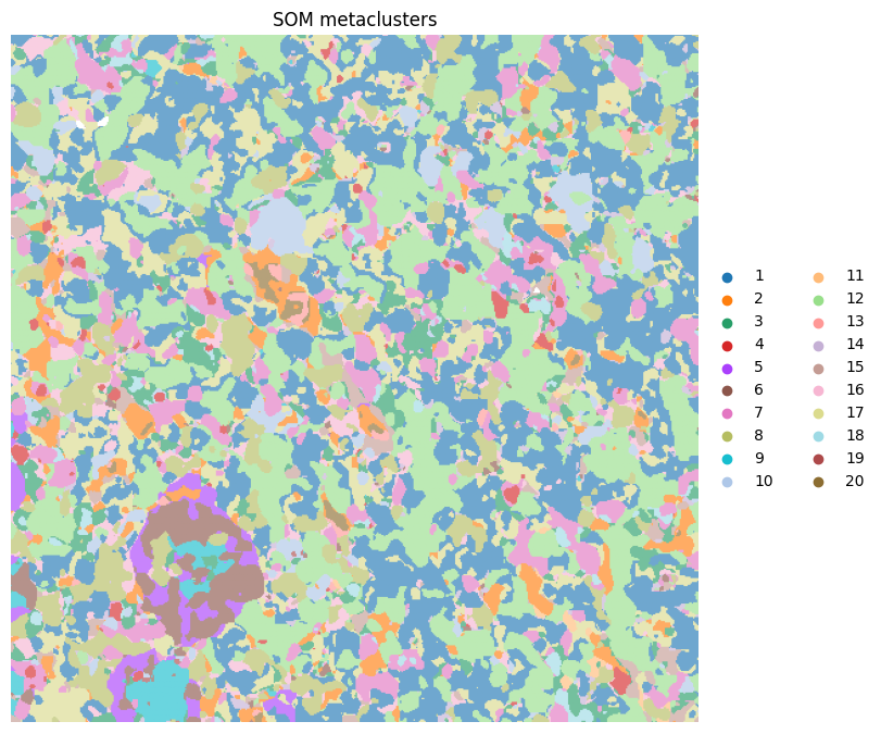
ax = hp.pl.pixel_clusters(
sdata,
labels_name="raw_image_fov0_flowsom_metaclusters",
figsize=(8, 8),
to_coordinate_system="fov0",
render_labels_kwargs={"alpha": 1},
title="SOM metaclusters",
)
ax.axis("off")
INFO     Dropping coordinate system 'fov9' since it doesn't have relevant elements.
INFO     Dropping coordinate system 'fov10' since it doesn't have relevant elements.
INFO     Dropping coordinate system 'fov1' since it doesn't have relevant elements.
INFO     Dropping coordinate system 'fov3' since it doesn't have relevant elements.
INFO     Dropping coordinate system 'fov7' since it doesn't have relevant elements.
INFO     Dropping coordinate system 'fov2' since it doesn't have relevant elements.
INFO     Dropping coordinate system 'fov6' since it doesn't have relevant elements.
INFO     Dropping coordinate system 'fov5' since it doesn't have relevant elements.
INFO     Dropping coordinate system 'fov8' since it doesn't have relevant elements.
INFO     Dropping coordinate system 'fov4' since it doesn't have relevant elements.
INFO     Successfully extracted 92 colors from 'cell_ID_cat_colors' in table
         '_value_clusters_d442b214-62cd-4feb-b8d5-2182bf62dc84'.
INFO     Dropping coordinate system 'fov9' since it doesn't have relevant elements.
INFO     Dropping coordinate system 'fov10' since it doesn't have relevant elements.
INFO     Dropping coordinate system 'fov1' since it doesn't have relevant elements.
INFO     Dropping coordinate system 'fov3' since it doesn't have relevant elements.
INFO     Dropping coordinate system 'fov7' since it doesn't have relevant elements.
INFO     Dropping coordinate system 'fov2' since it doesn't have relevant elements.
INFO     Dropping coordinate system 'fov6' since it doesn't have relevant elements.
INFO     Dropping coordinate system 'fov5' since it doesn't have relevant elements.
INFO     Dropping coordinate system 'fov8' since it doesn't have relevant elements.
INFO     Dropping coordinate system 'fov4' since it doesn't have relevant elements.
INFO     Successfully extracted 20 colors from 'cell_ID_cat_colors' in table
         '_value_clusters_f33730a1-d402-4580-a627-84de8a59afc6'.
(np.float64(0.0), np.float64(512.0), np.float64(512.0), np.float64(0.0))
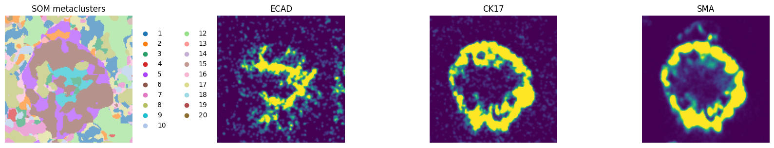
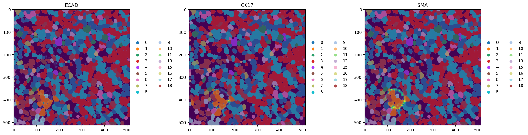
# visualize a crop:

fig, axes = plt.subplots(1, 4, figsize=(16, 4))

crd = [70, 210, 320, 460]

ax = hp.pl.pixel_clusters(
    sdata,
    labels_name="raw_image_fov0_flowsom_metaclusters",
    to_coordinate_system="fov0",
    ax=axes[0],
    render_labels_kwargs={"alpha": 1},
    crd=crd,
    title="SOM metaclusters",
)
ax.axis("off")

_image_name = "raw_image_fov0"
subset_channels = [
    "ECAD",
    "CK17",
    "SMA",
]

for _ax, _channel in zip(axes[1:], subset_channels, strict=True):
    # normalization parameters for visualization (underlying image not changed)
    se = hp.im.get_dataarray(sdata, element_name=_image_name)
    _channel_idx = np.where(sdata[_image_name].c.data == _channel)[0].item()
    vmax = da.percentile(se.data[_channel_idx].flatten(), q=99).compute()
    norm = Normalize(vmax=vmax, clip=False)

    render_images_kwargs = {"cmap": "viridis", "norm": norm}
    show_kwargs = {"title": _channel, "colorbar": False}
    _ax = hp.pl.plot_sdata(
        sdata,
        image_name=_image_name,
        to_coordinate_system="fov0",
        channel=_channel,
        crd=crd,
        render_images_kwargs=render_images_kwargs,
        show_kwargs=show_kwargs,
        ax=_ax,
    )
    # frameless figure
    _ax.axis("off")

plt.tight_layout()
plt.show()
INFO     Dropping coordinate system 'fov9' since it doesn't have relevant elements.
INFO     Dropping coordinate system 'fov10' since it doesn't have relevant elements.
INFO     Dropping coordinate system 'fov1' since it doesn't have relevant elements.
INFO     Dropping coordinate system 'fov3' since it doesn't have relevant elements.
INFO     Dropping coordinate system 'fov7' since it doesn't have relevant elements.
INFO     Dropping coordinate system 'fov2' since it doesn't have relevant elements.
INFO     Dropping coordinate system 'fov6' since it doesn't have relevant elements.
INFO     Dropping coordinate system 'fov5' since it doesn't have relevant elements.
INFO     Dropping coordinate system 'fov8' since it doesn't have relevant elements.
INFO     Dropping coordinate system 'fov4' since it doesn't have relevant elements.
INFO     Successfully extracted 19 colors from 'cell_ID_cat_colors' in table
         '_value_clusters_3288e2df-e5b4-48b0-8335-d37f0beb4618'.
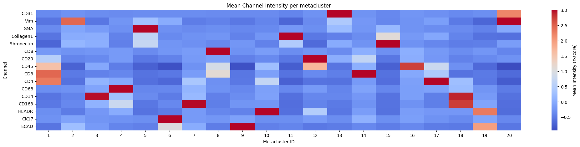
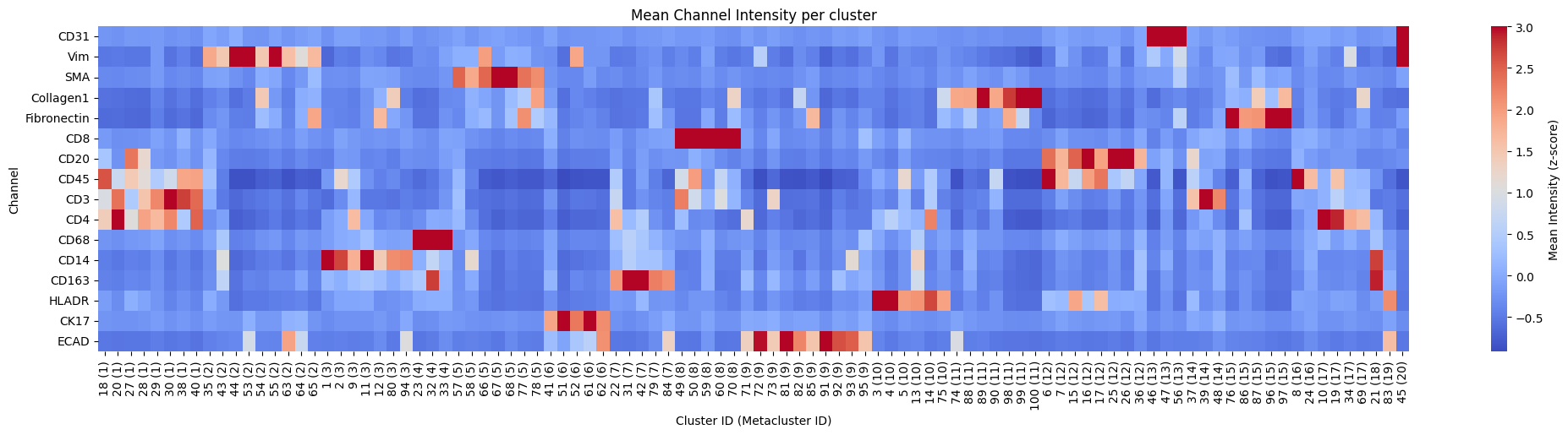
5. Heatmap of channel intensity per cluster and metacluster#
for _metaclusters in [True, False]:
    hp.pl.pixel_clusters_heatmap(
        sdata,
        table_name="counts_clusters",
        figsize=(25, 5),
        fig_kwargs={"dpi": 100},
        linewidths=0.001,
        metaclusters=_metaclusters,
        z_score=True,
    )
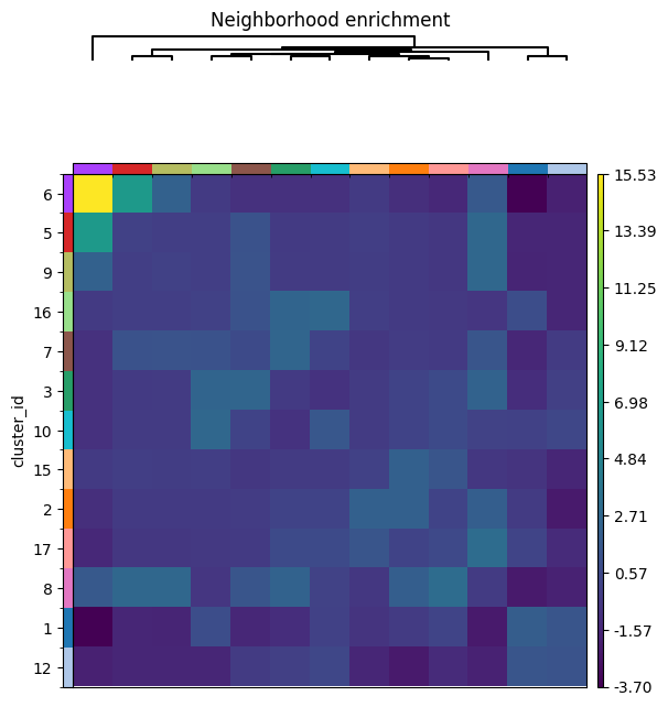
6. Spatial pixel neighbors#
import numpy as np
import squidpy as sq

key_added = "cluster_id"

adata = hp.tb.spatial_pixel_neighbors(
    sdata,
    labels_name="raw_image_fov0_flowsom_metaclusters",
    key_added=key_added,
    mode="most_frequent",
    grid_type="hexagon",
    size=20,
    subset=None,
)

adata.uns[f"{key_added}_nhood_enrichment"]["zscore"] = np.nan_to_num(
    adata.uns[f"{key_added}_nhood_enrichment"]["zscore"]
)
sq.pl.nhood_enrichment(
    adata, cluster_key=key_added, method="ward", mode="zscore", figsize=(6, 6)
)
INFO Creating graph using `grid` coordinates and `None` transform and `1` libraries.
7. Cell clustering#
batch_model = fs.models.BatchFlowSOMEstimator

table_name_flowsom_cell_clustering = "table_cell_clustering_flowsom"

sdata, fsom = hp.tb.flowsom(
    sdata,
    cells_labels_name=[
        f"label_whole_fov{i}" for i in range(N)
    ],  # segmentation masks, can be obtained using hp.im.segment.
    cluster_labels_name=[
        f"{_image_name}_flowsom_metaclusters" for _image_name in image_name
    ],  # here you could also choose  "raw_image_fov0_flowsom_clusters"
    output_table_name=table_name_flowsom_cell_clustering,
    chunks=512,
    model=batch_model,
    num_batches=10,
    random_state=100,
    overwrite=True,
)
Visualize the cell metaclusters:
fig, axes = plt.subplots(1, 3, figsize=(18, 6))
_image_name = "raw_image_fov0"
_labels_name = "label_whole_fov0"
subset_channels = ["ECAD", "CK17", "SMA"]

for _ax, _channel in zip(axes, subset_channels, strict=True):
    render_images_kwargs = {"cmap": "viridis", "norm": None}
    render_labels_kwargs = {"fill_alpha": 0.4, "outline_alpha": 0.4}
    show_kwargs = {"title": _channel, "colorbar": False}
    _ax = hp.pl.plot_sdata(
        sdata,
        image_name=_image_name,
        labels_name=_labels_name,
        table_name=table_name_flowsom_cell_clustering,
        color="metaclustering",
        channel=_channel,
        to_coordinate_system="fov0",
        render_images_kwargs=render_images_kwargs,
        render_labels_kwargs=render_labels_kwargs,
        show_kwargs=show_kwargs,
        ax=_ax,
    )
    # frameless figure
    # _ax.axis("off")

plt.tight_layout()
plt.show()
INFO     Successfully extracted 17 colors from 'metaclustering_colors' in table 'table_cell_clustering_flowsom'.
INFO     Successfully extracted 17 colors from 'metaclustering_colors' in table 'table_cell_clustering_flowsom'.
INFO     Successfully extracted 17 colors from 'metaclustering_colors' in table 'table_cell_clustering_flowsom'.
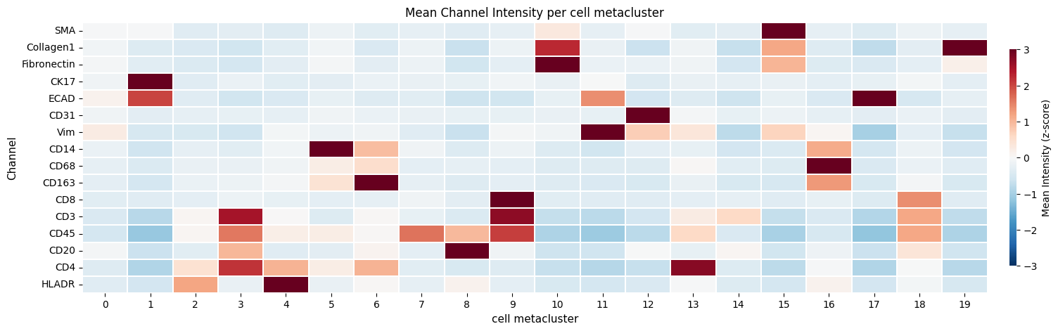
Now we want to visaulize the mean intensity per cell per cell metacluster, weighted by cell size. We first need to calculate the mean intensities per cell via hp.tb.allocate_intensitiy.
Note that in the ark pipeline, these intensities are weighted by the pixel SOM/META cluster count. To calculate these values, please use the harpy function hp.tb.weighted_channel_expression. Because for regular cell clustering, we only weight the intensities by the size of the cell, we choose to follow the same approach for Flowsom cell clustering.
labels_name = [f"label_whole_fov{i}" for i in range(N)]
to_coordinate_system = [f"fov{i}" for i in range(N)]
table_name = "table_intensities"

for i, (_image_name, _labels_name, _to_coordinate_system) in enumerate(
    zip(image_name, labels_name, to_coordinate_system, strict=True)
):
    sdata = hp.tb.allocate_intensity(
        sdata,
        image_name=_image_name,
        labels_name=_labels_name,
        channels=channels,
        output_table_name=table_name,
        mode="mean",
        to_coordinate_system=_to_coordinate_system,
        append=False if i == 0 else True,
        overwrite=True,
    )
The table element table contains annotated cluster information from the pixie pipeline (Liu, C.C., Greenwald, N.F., Kong, A., et al. (2023)), lets see how they compare to our predicted metaclusters.
We also compare the results with regular leiden clustering on the mean intensity values per cell.
import pandas as pd

from spatialdata.models import TableModel

instance_key = sdata[table_name].uns[TableModel.ATTRS_KEY][TableModel.INSTANCE_KEY]
region_key = sdata[table_name].uns[TableModel.ATTRS_KEY][TableModel.REGION_KEY_KEY]

df = (
    sdata["table"]
    .obs[["fov", "label", "cell_meta_cluster"]]
    .rename(
        columns={
            "fov": region_key,
            "label": instance_key,
            "cell_meta_cluster": "cell_type",
        }
    )
)

index = sdata[table_name].obs.index
sdata[table_name].obs = pd.merge(
    sdata[table_name].obs, df, how="inner", on=[instance_key, region_key]
)
sdata[table_name].obs.index = index
Now also add the calculated (via hp.tb.flowsom) cell metacluster and cluster ids to the table element 'table_intensities'.
columns = ["metaclustering", "clustering", instance_key, region_key]

index = sdata[table_name].obs.index
name = sdata[table_name].obs.index.name

sdata[table_name].obs = pd.merge(
    sdata[table_name].obs,
    sdata[table_name_flowsom_cell_clustering].obs[columns],
    on=[instance_key, region_key],
    how="left",  # left merge, because in table "table_cell_clustering_flowsom", we removed cells with no overlap with any pixel cluster
)
sdata[table_name].obs.index = index
sdata[table_name].obs.index.name = name

# back "table_intensities", now with metaclustering, clustering and cell_type in .obs to zarr
sdata = hp.tb.add_table(
    sdata,
    adata=sdata[table_name],
    output_table_name=table_name,
    region=[f"label_whole_fov{i}" for i in range(N)],
    overwrite=True,
)
sdata = hp.tb.cluster_intensity(
    sdata,
    table_name=table_name,
    labels_name=[f"label_whole_fov{i}" for i in range(N)],
    output_table_name=table_name,
    cluster_key="metaclustering",
    overwrite=True,
)

ax = hp.pl.cluster_intensity_heatmap(
    sdata,
    table_name=table_name,
    cluster_key="metaclustering",
    figsize=(20, 5),
)
ax.set_title("Mean Channel Intensity per cell metacluster")
_x_label = "cell metacluster"

ax.set_ylabel("Channel")
ax.set_xlabel(_x_label)
Text(0.5, 25.722222222222214, 'cell metacluster')
Now compare these results with regular leiden clustering on the mean intensity values.
# normalize before calculating leiden clusters

labels_name = [f"label_whole_fov{i}" for i in range(N)]

sdata = hp.tb.preprocess_proteomics(
    sdata,
    labels_name=labels_name,
    table_name=table_name,
    output_table_name=f"{table_name}_normalized",
    size_norm=False,
    log1p=False,
    q=0.99,
    max_value_q=1,
    overwrite=True,
)

sdata[f"{table_name}_normalized"].to_df().head()
| channels | CD3 | CD4 | CD8 | CD14 | CD20 | CD31 | CD45 | CD68 | CD163 | CK17 | Collagen1 | Fibronectin | ECAD | HLADR | SMA | Vim |
|---|---|---|---|---|---|---|---|---|---|---|---|---|---|---|---|---|
| cells | ||||||||||||||||
| 1_label_whole_fov0_09c64416 | 100.000000 | 96.655785 | 9.260165 | 6.321351 | 79.335533 | 0.000000 | 90.805908 | 6.274621 | 0.227555 | 1.503724 | 0.539386 | 1.673003 | 5.863480 | 6.114070 | 0.000000 | 8.542078 |
| 2_label_whole_fov0_09c64416 | 100.000000 | 100.000000 | 1.209254 | 100.000000 | 2.598548 | 1.285120 | 100.000000 | 12.967047 | 16.018177 | 8.001880 | 6.170453 | 0.884670 | 1.455017 | 43.258686 | 0.000000 | 3.866230 |
| 3_label_whole_fov0_09c64416 | 15.790016 | 85.442596 | 1.418018 | 12.311816 | 2.535572 | 1.271602 | 21.691730 | 0.000000 | 6.402584 | 2.490408 | 4.536551 | 6.552049 | 19.387783 | 67.727722 | 1.097208 | 9.684464 |
| 4_label_whole_fov0_09c64416 | 3.287402 | 28.842407 | 1.678827 | 4.460878 | 2.108853 | 0.098956 | 17.441771 | 53.642143 | 7.235740 | 15.314676 | 8.828622 | 6.231126 | 2.147254 | 7.351690 | 1.177836 | 3.420511 |
| 5_label_whole_fov0_09c64416 | 94.864815 | 100.000000 | 1.495612 | 16.172941 | 11.171283 | 2.316715 | 100.000000 | 13.128244 | 10.937386 | 18.826359 | 29.220844 | 22.919373 | 17.487209 | 43.814114 | 7.093751 | 15.714072 |
sdata = hp.tb.leiden(
    sdata,
    labels_name=labels_name,
    table_name=f"{table_name}_normalized",
    output_table_name=f"{table_name}_normalized",
    key_added="leiden",
    overwrite=True,
)
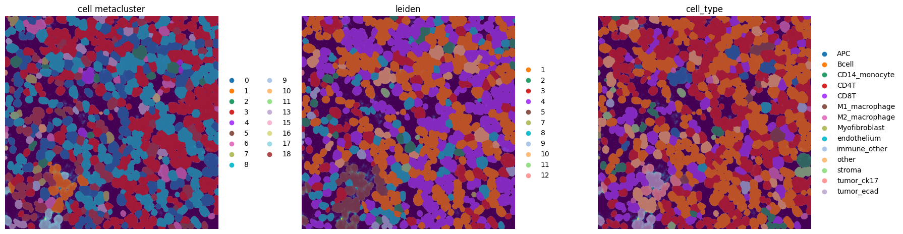
fig, axes = plt.subplots(1, 3, figsize=(18, 6))
_image_name = "raw_image_fov0"
subset_channels = ["ECAD", "CK17", "SMA"]

for _ax, _channel in zip(axes, subset_channels, strict=True):
    render_images_kwargs = {"cmap": "viridis", "norm": None}
    render_labels_kwargs = {"fill_alpha": 0.4, "outline_alpha": 0.4}
    show_kwargs = {"title": _channel, "colorbar": False}
    _ax = hp.pl.plot_sdata(
        sdata,
        image_name=_image_name,
        labels_name="label_whole_fov0",
        table_name=f"{table_name}_normalized",
        color="leiden",
        channel=_channel,
        to_coordinate_system="fov0",
        render_images_kwargs=render_images_kwargs,
        render_labels_kwargs=render_labels_kwargs,
        show_kwargs=show_kwargs,
        ax=_ax,
    )
    # frameless figure
    _ax.axis("off")

plt.tight_layout()
plt.show()
INFO     Successfully extracted 11 colors from 'leiden_colors' in table 'table_intensities_normalized'.
INFO     Successfully extracted 11 colors from 'leiden_colors' in table 'table_intensities_normalized'.
INFO     Successfully extracted 11 colors from 'leiden_colors' in table 'table_intensities_normalized'.
sdata = hp.tb.cluster_intensity(
sdata,
table_name=f"{table_name}_normalized",
labels_name=labels_name,
output_table_name=f"{table_name}_normalized",
cluster_key="leiden",
layer_mean_intensities="raw_counts", # layer in adata.layers that holds the mean intensities
overwrite=True,
)
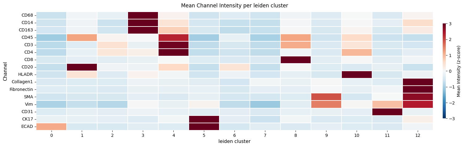
hp.pl.cluster_intensity_heatmap(
sdata,
table_name=f"{table_name}_normalized",
cluster_key="leiden",
figsize=(20, 5),
)
<Axes: title={'center': 'Mean Channel Intensity per leiden cluster'}, xlabel='leiden cluster', ylabel='Channel'>
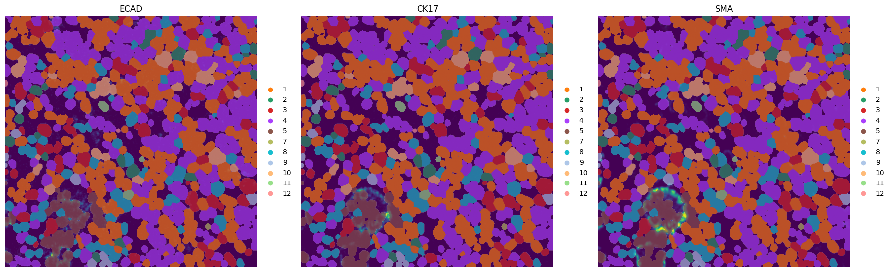
fig, axes = plt.subplots(1, 3, figsize=(18, 6))
_image_name = "raw_image_fov0"
_labels_name = "label_whole_fov0"
_to_coordinate_system = "fov0"
channel = "ECAD"

colors = ["metaclustering", "leiden", "cell_type"]

for _ax, _color in zip(axes, colors, strict=True):
    render_images_kwargs = {"cmap": "viridis", "norm": None}
    render_labels_kwargs = {"fill_alpha": 0.4, "outline_alpha": 0.4}
    show_kwargs = {
        "title": "cell metacluster" if _color == "metaclustering" else _color,
        "colorbar": False,
    }
    _ax = hp.pl.plot_sdata(
        sdata,
        image_name=_image_name,
        labels_name=_labels_name,
        table_name=f"{table_name}_normalized",
        color=_color,
        channel=channel,
        to_coordinate_system=_to_coordinate_system,
        render_images_kwargs=render_images_kwargs,
        render_labels_kwargs=render_labels_kwargs,
        show_kwargs=show_kwargs,
        ax=_ax,
    )
    # frameless figure
    _ax.axis("off")

plt.tight_layout()
plt.show()
INFO     Successfully extracted 17 colors from 'metaclustering_colors' in table 'table_intensities_normalized'.
INFO     Successfully extracted 11 colors from 'leiden_colors' in table 'table_intensities_normalized'.
INFO     Successfully extracted 14 colors from 'cell_type_colors' in table 'table_intensities_normalized'.
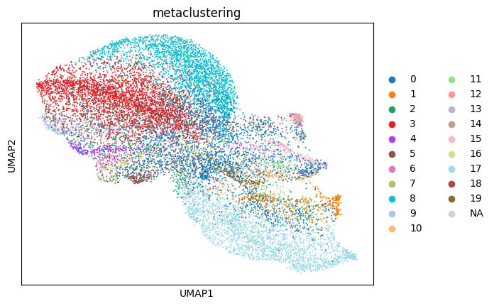
import scanpy as sc
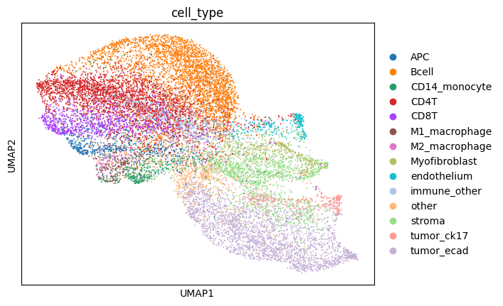
# note that these umaps are skwed towards the flowsom metaclusters, because cell type was annotated in Liu, C.C., Greenwald, N.F., Kong, A., et al. (2023) based on the flowsom cell metaclusters.
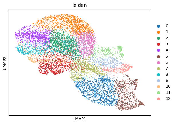
sc.pl.umap(sdata[f"{table_name}_normalized"], color=["metaclustering"])
sc.pl.umap(sdata[f"{table_name}_normalized"], color=["leiden"])
sc.pl.umap(sdata[f"{table_name}_normalized"], color=["cell_type"])
import matplotlib.pyplot as plt
import numpy as np
import pandas as pd
import seaborn as sns
from scipy.stats import chi2_contingency

table_name = "table_intensities_normalized"

for _cluster_key in ["metaclustering", "leiden"]:
    df = sdata[table_name].obs.copy()

    df = df[~df["cell_type"].isna()]

    contingency = pd.crosstab(df["cell_type"], df[_cluster_key])

    # chi squared test
    chi2, p, dof, expected = chi2_contingency(contingency)

    # cramers v
    def _cramers_v(confusion_matrix):
        chi2 = chi2_contingency(confusion_matrix)[0]
        n = confusion_matrix.sum().sum()
        phi2 = chi2 / n
        r, k = confusion_matrix.shape
        return np.sqrt(phi2 / min(k - 1, r - 1))

    print("Cramers v:", _cramers_v(contingency))

    print("Chi-squared statistic:", chi2)
    print("p-value:", p)

    plt.figure(figsize=(10, 5))
    sns.heatmap(contingency, cmap="viridis")
    plt.title(f"Cell type × {_cluster_key} association")
    plt.show()

    # Calculate standardized residuals
    residuals = (contingency - expected) / np.sqrt(expected)

    residuals_df = pd.DataFrame(
        residuals, index=contingency.index, columns=contingency.columns
    )

    resid_long = residuals_df.stack().reset_index()
    resid_long.columns = ["cell_type", _cluster_key, "std_residual"]

    # Sort by strength of deviation
    resid_long["abs_resid"] = resid_long["std_residual"].abs()
    top_effects = resid_long.sort_values("abs_resid", ascending=False).head(20)
    print(top_effects)

    plt.figure(figsize=(10, 5))
    sns.heatmap(residuals_df, center=0, cmap="coolwarm", annot=False)
    plt.title(f"Standardized residuals: cell_type × {_cluster_key}")
    plt.show()
Cramers v: 0.69991741063673
Chi-squared statistic: 97654.5324193182
p-value: 0.0
         cell_type metaclustering  std_residual   abs_resid
155  Myofibroblast             15    103.856744  103.856744
277     tumor_ecad             17     91.604831   91.604831
28           Bcell              8     87.202481   87.202481
4              APC              4     77.543951   77.543951
241     tumor_ck17              1     77.285909   77.285909
45   CD14_monocyte              5     77.060010   77.060010
172    endothelium             12     76.526940   76.526940
98            CD8T             18     75.466500   75.466500
126  M2_macrophage              6     73.204699   73.204699
116  M1_macrophage             16     72.479940   72.479940
63            CD4T              3     64.018750   64.018750
89            CD8T              9     61.189459   61.189459
2              APC              2     59.505149   59.505149
231         stroma             11     48.206569   48.206569
194   immune_other             14     46.467947   46.467947
230         stroma             10     35.677866   35.677866
220         stroma              0     32.002908   32.002908
239         stroma             19     29.632755   29.632755
183   immune_other              3     24.820278   24.820278
263     tumor_ecad              3    -22.402067   22.402067
Cramers v: 0.5964185759950482
Chi-squared statistic: 65462.96455749018
p-value: 0.0
         cell_type leiden  std_residual  abs_resid
60            CD8T      8     95.244502  95.244502
10             APC     10     91.814672  91.814672
115    endothelium     11     78.908615  78.908615
14           Bcell      1     72.854824  72.854824
169     tumor_ecad      0     66.835918  66.835918
43            CD4T      4     60.049037  60.049037
100  Myofibroblast      9     49.568946  49.568946
29   CD14_monocyte      3     48.177373  48.177373
174     tumor_ecad      5     44.836489  44.836489
155         stroma     12     42.461703  42.461703
119   immune_other      2     41.272904  41.272904
19           Bcell      6     39.881712  39.881712
41            CD4T      2     36.845028  36.845028
81   M2_macrophage      3     34.920952  34.920952
161     tumor_ck17      5     34.536849  34.536849
137          other      7     33.313912  33.313912
68   M1_macrophage      3     33.243298  33.243298
150         stroma      7     25.112493  25.112493
152         stroma      9     24.516440  24.516440
13           Bcell      0    -19.195630  19.195630
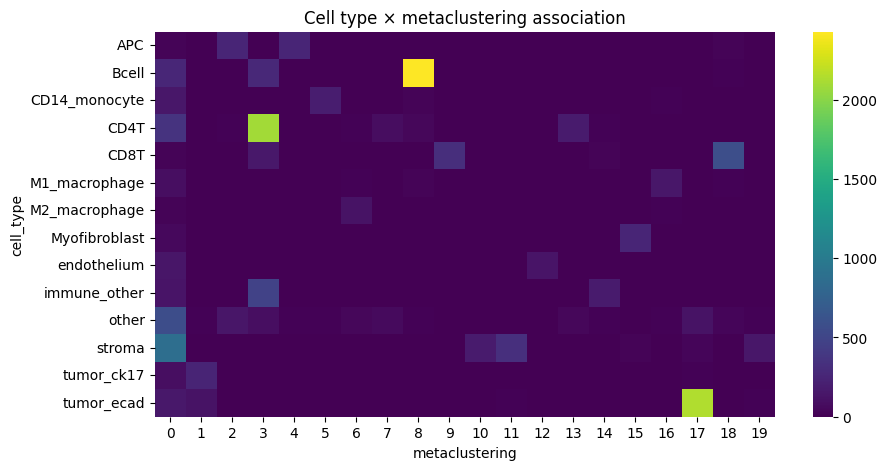
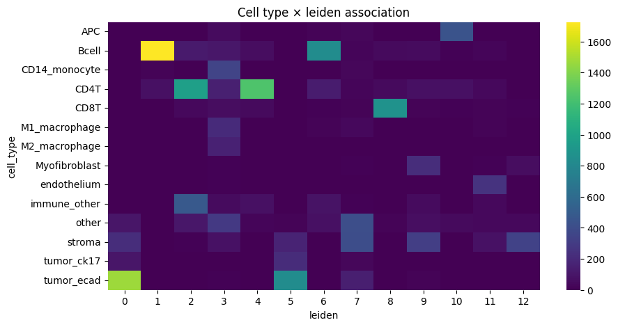
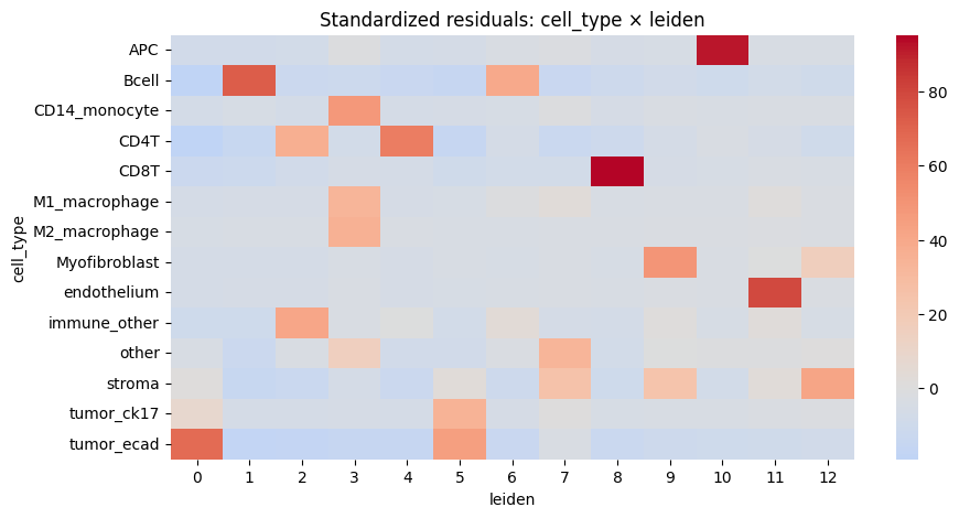
We notice a higher correlation between cell type predicted via cell metaclustering, compared to regular leiden clustering.
# "table_cell_clustering_flowsom" is annotated by segmentation masks, so they can also be visualised using napari-spatialdata
from spatialdata.models import TableModel

sdata["table_cell_clustering_flowsom"].uns[TableModel.ATTRS_KEY]

# from napari_spatialdata import Interactive

# Interactive(sdata)
{'region': ['label_whole_fov0',
  'label_whole_fov1',
  'label_whole_fov2',
  'label_whole_fov3',
  'label_whole_fov4',
  'label_whole_fov5',
  'label_whole_fov6',
  'label_whole_fov7',
  'label_whole_fov8',
  'label_whole_fov9',
  'label_whole_fov10'],
 'instance_key': 'cell_ID',
 'region_key': 'fov_labels'}
Optional export to a .csv format that can be used for visualization using the ark analysis gui#
# weighted channel average for visualization in the ark analysis gui (optional) -> calculate this on the flowsom clustered matrix
sdata = hp.tb.weighted_channel_expression(
    sdata,
    cell_clustering_table_name="table_cell_clustering_flowsom",
    table_name_pixel_cluster_intensity="counts_clusters",
    output_table_name="table_cell_clustering_flowsom",
    clustering_key=ClusteringKey._METACLUSTERING_KEY,
    overwrite=True,
)
from harpy.table.cell_clustering._utils import (
    _export_to_ark_format as _export_to_ark_format_cells,
)
from harpy.table.pixel_clustering._cluster_intensity import (
    _export_to_ark_format as _export_to_ark_format_pixels,
)

df = _export_to_ark_format_pixels(adata=sdata["counts_clusters"], output=None)
(
    df_cell_som_cluster_count_avg,
    df_cell_som_cluster_channel_avg,
    df_cell_meta_cluster_channel_avg,
) = _export_to_ark_format_cells(
    sdata, table_name="table_cell_clustering_flowsom", output=None
)
df.head()
| channels | CD3 | CD4 | CD8 | CD14 | CD20 | CD31 | CD45 | CD68 | CD163 | CK17 | Collagen1 | Fibronectin | ECAD | HLADR | SMA | Vim | pixel_meta_cluster | pixel_som_cluster | count |
|---|---|---|---|---|---|---|---|---|---|---|---|---|---|---|---|---|---|---|---|
| SOM_cluster_ID_index | |||||||||||||||||||
| 1_counts_clusters_4a0295d3 | 3.170556 | 12.888708 | 2.673701 | 102.297302 | 1.981421 | 1.010174 | 15.915800 | 5.115088 | 13.101303 | 1.311709 | 7.427465 | 6.707138 | 3.581628 | 7.404450 | 2.121363 | 3.902526 | 3 | 1 | 61858.0 |
| 2_counts_clusters_4a0295d3 | 7.802601 | 15.197968 | 5.868374 | 52.094273 | 6.514609 | 2.945678 | 43.575554 | 6.603859 | 11.311961 | 2.333262 | 7.480127 | 5.921785 | 3.862716 | 10.003304 | 2.255558 | 7.188983 | 3 | 2 | 76777.0 |
| 3_counts_clusters_4a0295d3 | 8.591969 | 18.529282 | 5.463168 | 7.904346 | 4.000842 | 1.638508 | 19.988863 | 6.152431 | 7.790992 | 2.215147 | 7.164235 | 5.330628 | 4.973933 | 78.794853 | 1.134772 | 11.190743 | 10 | 3 | 101431.0 |
| 4_counts_clusters_4a0295d3 | 6.426503 | 24.199673 | 3.257826 | 4.316765 | 1.848322 | 0.914533 | 15.558946 | 3.096722 | 4.072947 | 1.105101 | 4.323403 | 2.858347 | 2.538521 | 117.102592 | 0.420902 | 5.771106 | 10 | 4 | 59752.0 |
| 5_counts_clusters_4a0295d3 | 16.677263 | 19.242825 | 9.086171 | 8.071563 | 7.421441 | 2.405537 | 43.708309 | 5.483037 | 7.129220 | 3.141083 | 6.394245 | 4.868136 | 4.656443 | 43.941631 | 1.605118 | 9.540346 | 10 | 5 | 85247.0 |
df_cell_meta_cluster_channel_avg.head()
| cell_meta_cluster | CD3 | CD4 | CD8 | CD14 | CD20 | CD31 | CD45 | CD68 | CD163 | CK17 | Collagen1 | Fibronectin | ECAD | HLADR | SMA | Vim | cell_meta_cluster_rename | |
|---|---|---|---|---|---|---|---|---|---|---|---|---|---|---|---|---|---|---|
| 0 | 1 | 13.312110 | 14.540046 | 5.212882 | 10.652877 | 9.342804 | 4.176129 | 19.527418 | 5.825487 | 8.925391 | 4.812573 | 13.868835 | 12.002700 | 10.981284 | 8.484389 | 5.987512 | 19.682054 | 1 |
| 1 | 2 | 6.822442 | 6.668731 | 4.851417 | 7.685502 | 3.745090 | 2.177237 | 6.608780 | 3.866220 | 8.094399 | 32.722800 | 11.086600 | 10.109598 | 32.357767 | 5.390016 | 3.112652 | 15.338476 | 2 |
| 2 | 3 | 15.606988 | 23.245666 | 5.825461 | 10.316361 | 6.800073 | 2.170474 | 24.766719 | 6.335626 | 9.973863 | 3.105719 | 10.342049 | 7.480709 | 9.202182 | 33.578242 | 2.408904 | 10.282013 | 3 |
| 3 | 4 | 40.002591 | 39.067493 | 6.690993 | 6.638652 | 13.699744 | 2.078078 | 41.266476 | 4.937002 | 7.077583 | 3.187016 | 6.369957 | 4.418863 | 3.123610 | 8.655178 | 2.144527 | 8.340994 | 4 |
| 4 | 5 | 12.083061 | 23.661401 | 5.614998 | 11.034528 | 4.662411 | 1.841157 | 24.230448 | 6.375871 | 9.522896 | 2.408798 | 10.240973 | 7.033974 | 4.482985 | 54.909245 | 1.879081 | 9.668706 | 5 |