Rasterize and vectorize

This tutorial illustrates how to convert a segmentation mask (array) into its vectorized form, and segmentation boundaries (polygons) into their rasterized equivalents. This conversion is useful, for example, when integrating annotations (e.g., from QuPath) into downstream spatial omics analysis.

For raster-to-vector conversion, we provide the function harpy.sh.vectorize, and for vector-to-raster conversion, we provide the function harpy.im.rasterize. These functions transform a labels element (raster) in a SpatialData object into a shapes element (polygons), and vice versa. They also manage coordinate systems and related transformations defined on the spatial elements automatically.

The harpy.sh.vectorize internally relies on the rasterio library, while harpy.im.rasterize uses Datashader. Both functions are optimized with Dask for multi-core and out-of-core processing.

1. Example on dummy data

from spatialdata.datasets import blobs

sdata = blobs(length=1000, n_channels=3)

Let’s perform the following conversions: raster → vector → raster → vector, and check whether the results are consistent.

import harpy as hp

sdata = hp.sh.vectorize(
    sdata,
    labels_name="blobs_labels",
    output_shapes_name="blobs_labels_boundaries",
    overwrite=True,
)

sdata = hp.im.rasterize(
    sdata,
    shapes_name="blobs_labels_boundaries",
    output_labels_name="blobs_labels_redo",
    chunks=1000,
    overwrite=True,
)

sdata = hp.sh.vectorize(
    sdata,
    labels_name="blobs_labels_redo",
    output_shapes_name="blobs_labels_boundaries_redo",
    overwrite=True,
)

We proceed to show that they are in fact equal:

display(sdata["blobs_labels_boundaries"].head())
display(sdata["blobs_labels_boundaries_redo"].head())

	geometry
cell_ID
1	MULTIPOLYGON (((801 41, 801 40, 800 40, 800 41...
2	MULTIPOLYGON (((681 591, 681 590, 680 590, 680...
3	POLYGON ((335 338, 335 339, 331 339, 331 341, ...
4	POLYGON ((181 600, 181 601, 176 601, 176 602, ...
5	MULTIPOLYGON (((429 267, 426 267, 426 268, 423...

	geometry
cell_ID
1	MULTIPOLYGON (((801 41, 801 40, 800 40, 800 41...
2	MULTIPOLYGON (((681 591, 681 590, 680 590, 680...
3	POLYGON ((335 338, 335 339, 331 339, 331 341, ...
4	POLYGON ((181 600, 181 601, 176 601, 176 602, ...
5	MULTIPOLYGON (((429 267, 426 267, 426 268, 423...

import numpy as np

assert np.array_equal(sdata["blobs_labels"].data.compute(), sdata["blobs_labels_redo"].data.compute())
assert sdata["blobs_labels_boundaries"].geometry.equals(sdata["blobs_labels_boundaries_redo"].geometry)

And finally a visual inspection.

import matplotlib.pyplot as plt

fig, axes = plt.subplots(1, 2, figsize=(8, 4))

channel = 0

render_images_kwargs = {"cmap": "binary"}

for _labels_name, ax in zip(["blobs_labels", "blobs_labels_redo"], axes, strict=True):
    render_labels_kwargs = {"fill_alpha": 0.6, "outline_alpha": 0.4}
    show_kwargs = {
        "title": "DAPI",
        "colorbar": False,
    }

    show_kwargs = {
        "title": _labels_name,
        "colorbar": False,
    }
    ax = hp.pl.plot_sdata(
        sdata,
        image_name="blobs_image",
        labels_name="blobs_labels",
        channel=0,
        render_images_kwargs=render_images_kwargs,
        render_labels_kwargs=render_labels_kwargs,
        show_kwargs=show_kwargs,
        ax=ax,
    )
    ax.axis("off")

plt.tight_layout()
plt.show()

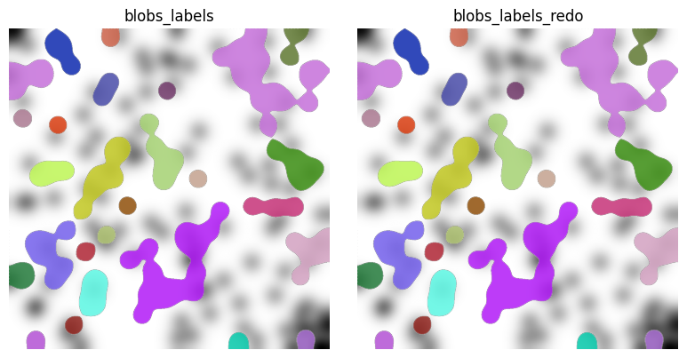
Be advised that the transformation from raster to polygon formats, or vice versa, can yield small deviations attributable to numerical precision limitations.

2. Example on MERSCOPE data.

import harpy as hp

sdata = hp.datasets.merscope_mouse_liver_segmentation_mask()

We perform a roundtrip, raster → vector → raster, and visually check whether the resulting rasters look the same.

import dask

labels_name = "segmentation_mask_full"
shapes_name = "segmentation_mask_full_boundaries"

dask.config.set(scheduler="processes")

# takes 1m40 on MacOS (m2)
sdata = hp.sh.vectorize(
    sdata,
    labels_name=labels_name,
    output_shapes_name=shapes_name,
    overwrite=True,
)

print("Finished vectorizing.")

# latter code consumes a lot of ram because sdata is not backed in this example.
# back sdata to zarr store for low ram consumption

# set to threads for efficient processing, or define a dask client using few workers and threads.
dask.config.set(scheduler="threads")

# takes around 1m30 on MacOS (m2)
sdata = hp.im.rasterize(
    sdata,
    shapes_name=shapes_name,
    output_labels_name=labels_name + "_redo",
    chunks=5000,
    overwrite=True,
)

print("Finished rasterizing.")

Finished vectorizing.
Finished rasterizing.

Visual inspection.

import matplotlib.pyplot as plt

image_name = "clahe"
labels_name = "segmentation_mask_full"

fig, axes = plt.subplots(1, 2, figsize=(16, 8))

channel = 0

render_images_kwargs = {"cmap": "binary"}
render_labels_kwargs = {"fill_alpha": 0.6, "outline_alpha": 0.4}

for _labels_name, ax in zip(["segmentation_mask_full", "segmentation_mask_full_redo"], axes, strict=True):
    # subset, because query is slow on points element
    sdata_to_plot = sdata.subset(element_names=[image_name, _labels_name])

    color = channel
    show_kwargs = {
        "title": "Segmentation mask" if _labels_name == "segmentation_mask_full" else "Segmentation mask redo",
        "colorbar": False,
    }
    ax = hp.pl.plot_sdata(
        sdata_to_plot,
        image_name=image_name,
        channel=channel,
        labels_name=_labels_name,
        crd=[20000, 30000, 20000, 30000],
        render_images_kwargs=render_images_kwargs,
        render_labels_kwargs=render_labels_kwargs,
        show_kwargs=show_kwargs,
        to_coordinate_system="global",
        ax=ax,
    )
    ax.axis("off")

plt.tight_layout()
plt.show()

INFO     Rasterizing image for faster rendering.                                                                   
INFO     Rasterizing image for faster rendering.                                                                   
INFO     Rasterizing image for faster rendering.                                                                   
INFO     Rasterizing image for faster rendering.

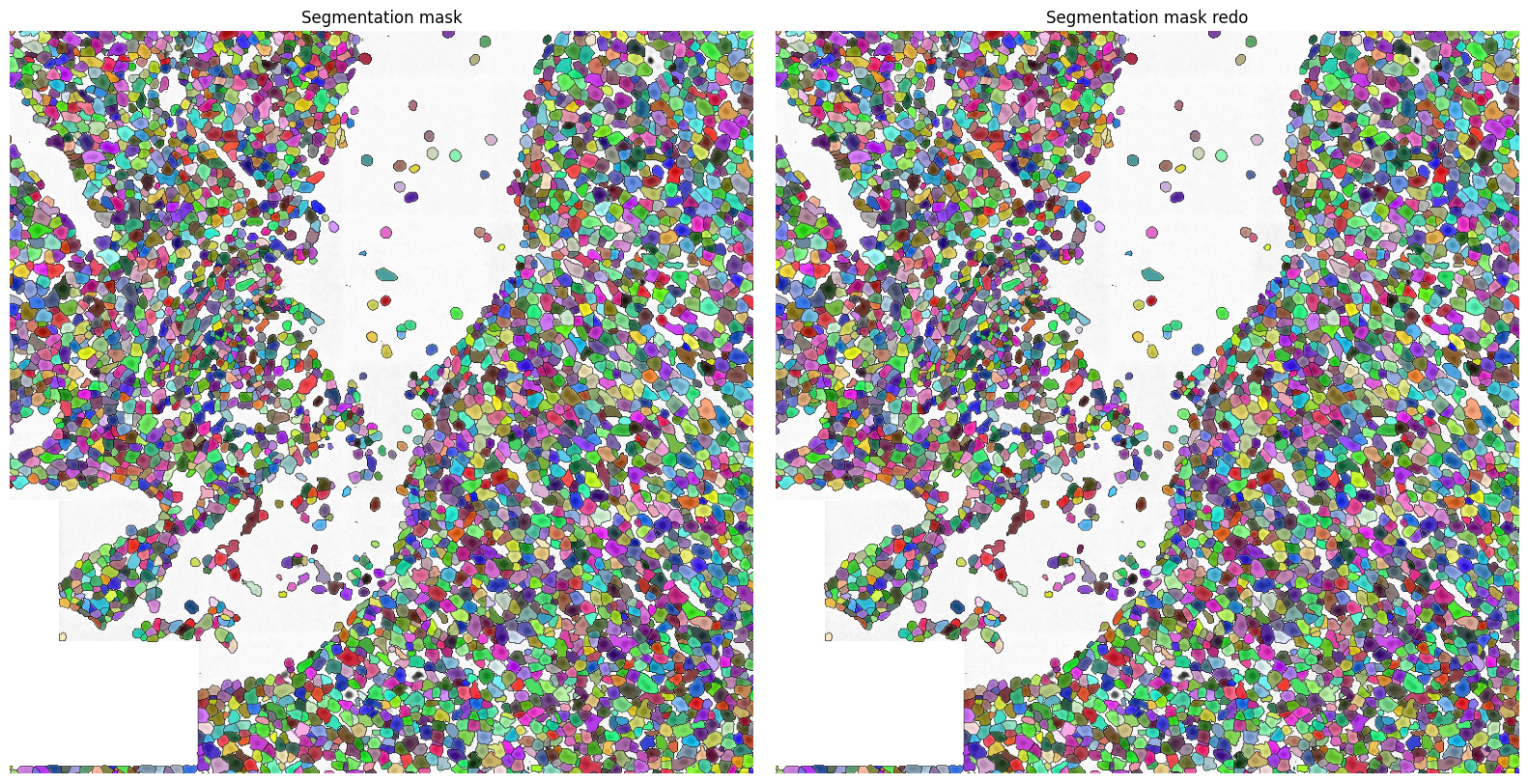
Again, both segmentation masks look very similar.