Scalable Spatial Transcriptomics Analysis with Harpy.

# installation:
uv venv .venv_harpy_cellpose_3 --python 3.12
source .venv_harpy_cellpose_3/bin/activate
uv pip install "harpy-analysis[extra]"
uv pip install squidpy
uv pip install cellpose==3.1.1.3
uv pip install jupyter

Introduction

Harpy is a spatial omics analysis library built to work naturally with SpatialData and downstream tools such as AnnData, Scanpy, and Squidpy. It focuses on the scalable computational parts of a spatial workflow, especially when working with large images and large spatial omics datasets.

In practice, Harpy provides fast, out-of-core image preprocessing, scalable tiled segmentation, and efficient aggregation workflows to create AnnData tables and calculate per-cell features from images, labels, shapes, and transcript coordinates.

A helpful way to think about Harpy is as a scalable computational layer on top of SpatialData: SpatialData organizes and stores the spatial elements, while Harpy performs the heavy computation on them and returns results in standard data structures that integrate well with the broader Python single-cell and spatial analysis stack.

This notebook illustrates that role end to end: we use Harpy to read and manage spatial data, preprocess large images, run segmentation, create transcriptomics and proteomics-style AnnData tables, compute transcript and instance density maps, and then continue with familiar downstream tools such as Scanpy and Squidpy for preprocessing, clustering, annotation, and visualization.

import spatialdata_plot

import harpy as hp

_ = spatialdata_plot

1. Fetch the SpatialData object

This notebook uses a subset of the 10x Genomics Xenium Prime FFPE human ovarian cancer dataset to keep the workflow lighter to run. We also analyzed the full dataset, for that version, see this notebook.

Xenium already provides a segmentation mask and an AnnData table, but in this notebook we want to illustrate how segmentation can be obtained with Harpy, and how the AnnData table can be created. In practice, rerunning segmentation is often worthwhile: different tissues and special cell types can require different settings, segmentation quality can often be improved by tuning the model and preprocessing steps. Accurate segmentation is known to be essential for strong downstream results because it directly affects transcript assignment and all per-cell measurements.

To keep the workflow lightweight and focused on the relevant inputs, we subset the SpatialData object and retain only the layers that we use downstream. In practice, we keep the morphology and H&E images together with the transcript points, and discard the remaining elements before continuing with preprocessing and segmentation.

If you want to read a Xenium dataset with Harpy directly, you can use hp.io.xenium(...). If you request to_coordinate_system="global", then global corresponds to the pixel coordinate system and Harpy will also add global_micron as the micron coordinate system by default. The simplest way to back the imported object to disk is to pass an output path, which writes the result to a Zarr store while reading:

'''
import harpy as hp
from spatialdata import read_zarr

zarr_path = "/path/to/sdata.zarr"

sdata = hp.io.xenium(
    "/path/to/xenium_sample",
    to_coordinate_system="global",
    aligned_images=True,
    cells_table=True,
    nucleus_labels=True,
    cells_labels=True,
    output=zarr_path,
)
'''

import tempfile
from pathlib import Path

import geopandas as gpd
from spatialdata import read_zarr

from harpy.datasets.registry import get_registry

registry_path = None

spatialdata_path = Path(tempfile.mkdtemp()) / "sdata.zarr"

sdata = hp.datasets.xenium_human_ovarian_cancer(
    subset=True, processed=False, path=registry_path
)

elements_to_keep = [
    "he_image_global",
    "morphology_focus_global",
    "transcripts_global",
]

for _element in (
    [*sdata.images]
    + [*sdata.labels]
    + [*sdata.shapes]
    + [*sdata.tables]
    + [*sdata.points]
):
    if _element not in elements_to_keep:
        del sdata[_element]

sdata.write(spatialdata_path, overwrite=True)
sdata = read_zarr(sdata.path)

# Normalize channel names
channel_names = hp.im.get_dataarray(
    sdata, element_name="morphology_focus_global"
).c.data
sdata.set_channel_names(
    element_name="morphology_focus_global",
    channel_names=[_name.replace("/", "_") for _name in channel_names],
    write=True,
)

sdata = read_zarr(sdata.path)

registry = get_registry(path=registry_path)

# Lets add region annotations.
paths_to_GeoJSONs = {
    "tumor": registry.fetch(
        "transcriptomics/xenium/Xenium_human_ovarian_cancer/training_march_2026/tumor.geojson"
    ),
    "necrosis": registry.fetch(
        "transcriptomics/xenium/Xenium_human_ovarian_cancer/training_march_2026/necrosis.geojson"
    ),
    "ovary": registry.fetch(
        "transcriptomics/xenium/Xenium_human_ovarian_cancer/training_march_2026/ovary.geojson"
    ),
    "fallopian_tube": registry.fetch(
        "transcriptomics/xenium/Xenium_human_ovarian_cancer/training_march_2026/fallopian_tube.geojson"
    ),
    "smooth_muscle": registry.fetch(
        "transcriptomics/xenium/Xenium_human_ovarian_cancer/training_march_2026/smooth_muscle.geojson"
    ),
}

for name, path in paths_to_GeoJSONs.items():
    gdf_regions = gpd.read_file(path)
    sdata = hp.sh.add_shapes(
        sdata, input=gdf_regions, output_shapes_name=name, overwrite=True
    )

sdata

SpatialData object, with associated Zarr store: /private/var/folders/sz/t3tgg4fs4tz9btm0fbqg_tzc0000gn/T/tmpplr6sg2j/sdata.zarr
├── Images
│     ├── 'he_image_global': DataTree[cyx] (3, 7820, 7820), (3, 3910, 3910), (3, 1955, 1954), (3, 978, 977), (3, 489, 489)
│     └── 'morphology_focus_global': DataTree[cyx] (4, 10000, 10000), (4, 5000, 5000), (4, 2499, 2500), (4, 1249, 1250), (4, 624, 625)
├── Points
│     └── 'transcripts_global': DataFrame with shape: (<Delayed>, 3) (2D points)
└── Shapes
      ├── 'fallopian_tube': GeoDataFrame shape: (1, 3) (2D shapes)
      ├── 'necrosis': GeoDataFrame shape: (15, 3) (2D shapes)
      ├── 'ovary': GeoDataFrame shape: (3, 3) (2D shapes)
      ├── 'smooth_muscle': GeoDataFrame shape: (1, 3) (2D shapes)
      └── 'tumor': GeoDataFrame shape: (3, 3) (2D shapes)
with coordinate systems:
    ▸ 'global', with elements:
        he_image_global (Images), morphology_focus_global (Images), transcripts_global (Points), fallopian_tube (Shapes), necrosis (Shapes), ovary (Shapes), smooth_muscle (Shapes), tumor (Shapes)
    ▸ 'global_micron', with elements:
        he_image_global (Images), morphology_focus_global (Images), transcripts_global (Points)

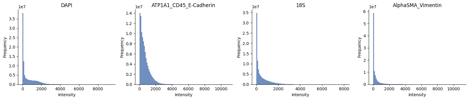
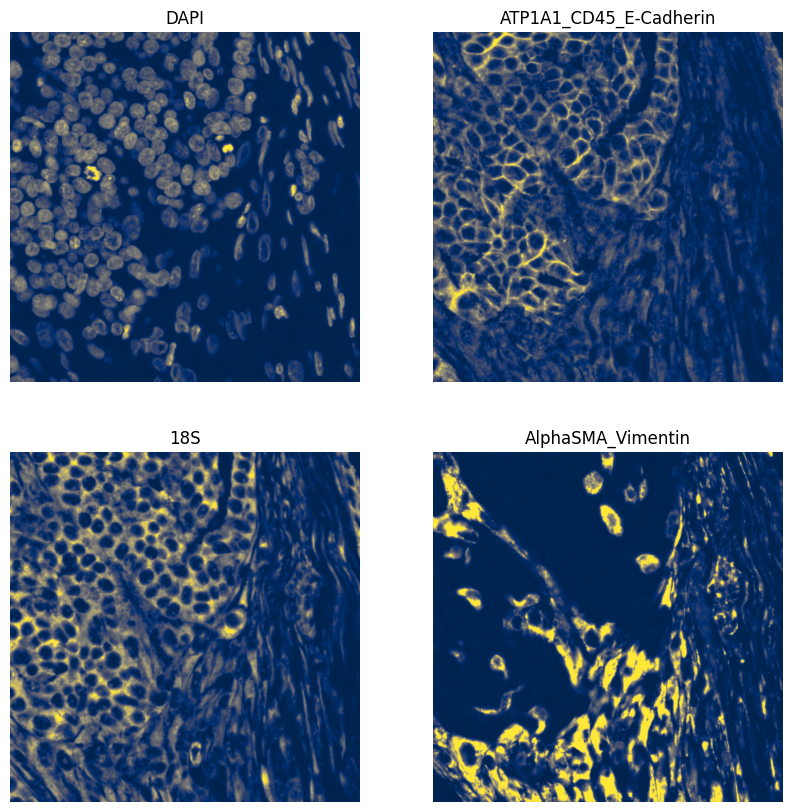
2. Image preprocessing

To improve segmentation quality, we have several options to first preprocess the images to improve the quality, contrast, remove background, etc. This can help to get much better segmentation masks, but note that in many cases (depending on the exact combination of image quality, tissue type and segmentation model), we can safely skip this step and get good results with just the raw images.

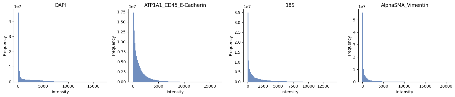
channels = hp.im.get_dataarray(sdata, element_name="morphology_focus_global").c.data

ax = hp.qc.image_histogram(
    sdata,
    image_name="morphology_focus_global",
    channel=channels,
    density=False,
    ncols=4,
    bins=100,
)

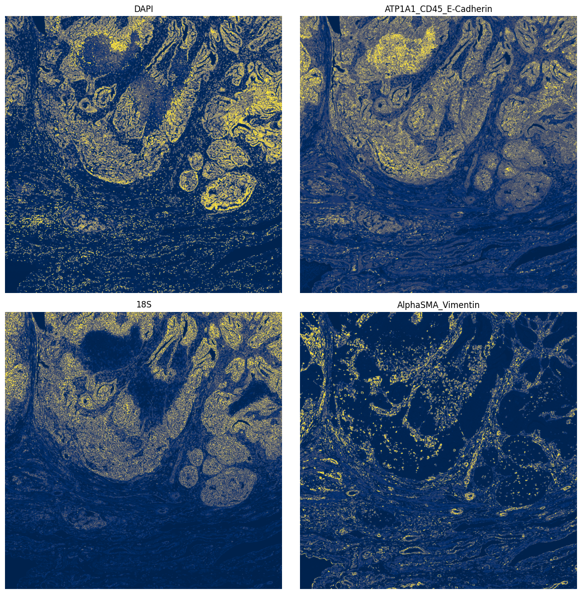
import matplotlib.pyplot as plt
from matplotlib.colors import Normalize

fig, axes = plt.subplots(2, 2, figsize=(12, 12))
_image_name = "morphology_focus_global"
to_coordinate_system = "global"

for ax, _channel in zip(axes.flatten(), channels, strict=True):
    norm = Normalize(vmin=0, vmax=2500)

    render_images_kwargs = {"cmap": "cividis", "norm": norm}
    show_kwargs = {"title": _channel, "colorbar": False}
    ax = hp.pl.plot_sdata(
        sdata,
        image_name=_image_name,
        channel=_channel,
        to_coordinate_system=to_coordinate_system,
        render_images_kwargs=render_images_kwargs,
        show_kwargs=show_kwargs,
        ax=ax,
    )
    # frameless figure
    ax.axis("off")

plt.tight_layout()
plt.show()

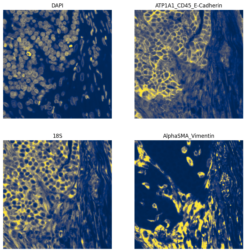
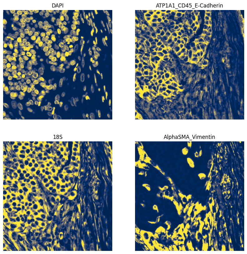
2.1 Min-max filtering and contrast enhancing

The next preprocessing steps include:

• A min max filter can be added. The goal of this function is to substract background noise and make the borders of the nuclei/cells cleaner. It will also remove some debris. Note that if you set the size of the filter too small (smaller then the size of your nuclei), the function will create “donuts” (black spots in the center of your cells). If the size of the min max filter is chosen too big, not enough background will be subtracted. Generally, you want to aim for the average nucleus size and some fine-tuning may be necessary.

• We also recommend to perform contrast enhancement on your image. Harpy does this by using histogram equalization (CLAHE function). The amount of correction needed can be decided by adapting the contrast_clip value. If the image is already quite bright, 3.5 might be a good starting point. For dark images, you can go up to 10 or even more. Make sure at the end the whole image is evenly illuminated and no cells are dark in the background.

If you think your data needs further image processing steps, you can perform these using the map_image function (see further).

# First, we plot the raw images for comparison
fig, axes = plt.subplots(2, 2, figsize=(10, 10))

for ax, channel in zip(axes.ravel(), channels, strict=True):
    norm = Normalize(vmin=0, vmax=3000)

    ax = hp.pl.plot_sdata(
        sdata,
        image_name="morphology_focus_global",
        channel=channel,
        crd=(10000, 11000, 18000, 19000),
        to_coordinate_system="global",
        render_images_kwargs={"cmap": "cividis", "norm": norm},
        show_kwargs={"title": channel, "colorbar": False},
        ax=ax,
    )
    ax.axis("off")

# Perform min max filtering
sdata = hp.im.min_max_filtering(
    sdata,
    image_name="morphology_focus_global",
    output_image_name="min_max_filtered",
    size_min_max_filter=55,
    overwrite=True,
)

# Plot min-max filtered images
fig, axes = plt.subplots(2, 2, figsize=(10, 10))

for ax, channel in zip(axes.ravel(), channels, strict=True):
    norm = Normalize(vmin=0, vmax=3000)

    ax = hp.pl.plot_sdata(
        sdata,
        image_name="min_max_filtered",
        channel=channel,
        crd=(10000, 11000, 18000, 19000),
        to_coordinate_system="global",
        render_images_kwargs={"cmap": "cividis", "norm": norm},
        show_kwargs={"title": channel, "colorbar": False},
        ax=ax,
    )
    ax.axis("off")

# Perform contrast enhancement using OpenCV ( https://opencv.org/, cv2.createCLAHE )
sdata = hp.im.enhance_contrast(
    sdata,
    image_name="min_max_filtered",
    output_image_name="clahe",
    contrast_clip=2.5,
    chunks=3000,
    overwrite=True,
)


# plot the histogram
channels = hp.im.get_dataarray(sdata, element_name="clahe").c.data

ax = hp.qc.image_histogram(
    sdata,
    image_name="clahe",
    channel=channels,
    density=False,
    ncols=4,
    bins=100,
)

# Plot contrast enhanced images
fig, axes = plt.subplots(2, 2, figsize=(10, 10))

for ax, channel in zip(axes.ravel(), channels, strict=True):
    norm = Normalize(vmin=0, vmax=5000)

    ax = hp.pl.plot_sdata(
        sdata,
        image_name="clahe",
        channel=channel,
        crd=(10000, 11000, 18000, 19000),
        to_coordinate_system="global",
        render_images_kwargs={"cmap": "cividis", "norm": norm},
        show_kwargs={"title": channel, "colorbar": False},
        ax=ax,
    )
    ax.axis("off")

2.2 ADVANCED: Custom distributed preprocessing of images using hp.im.map_image and Dask

See https://docs.dask.org/en/stable/generated/dask.array.map_blocks.html and https://docs.dask.org/en/latest/generated/dask.array.map_overlap.html

Set blockwise==True if you want to do distributed processing using dask.array.map_blocks or dask.array.map_overlap, set blockwise==False if your function is already distributed (e.g. when using dask_image filters https://image.dask.org/en/latest/dask_image.ndfilters.html.)

import numpy as np
from numpy.typing import NDArray


# Define your custom function
def _my_dummy_function(image: NDArray, parameter: int | float) -> NDArray:
    # input (1,1,y,x)
    # output (1,1,y,x)
    print(f"Type of the image is: {type(image)}")
    print(image.shape)
    return image * parameter


fn_kwargs = {"parameter": 2}

# Apply custom function
sdata = hp.im.map_image(
    sdata,
    func=_my_dummy_function,
    fn_kwargs=fn_kwargs,
    image_name="morphology_focus_global",
    output_image_name="dummy_image",
    chunks=2048,
    blockwise=False,  # if blockwise == True --> input to _my_dummy_function is a numpy array of size chunks, else it is a Dask array (with chunksize chunks)
    depth=1000,  # if blockwise == True, and depth specified, will use map_overlap instead of map_blocks for distributed processing
    overwrite=True,
    dtype=np.uint16,
    meta=np.array((), dtype=np.uint16),
)

Type of the image is: <class 'dask.array.core.Array'>
(1, 1, 10000, 10000)
Type of the image is: <class 'dask.array.core.Array'>
(1, 1, 10000, 10000)
Type of the image is: <class 'dask.array.core.Array'>
(1, 1, 10000, 10000)
Type of the image is: <class 'dask.array.core.Array'>
(1, 1, 10000, 10000)

del sdata["dummy_image"]
sdata.delete_element_from_disk("dummy_image")

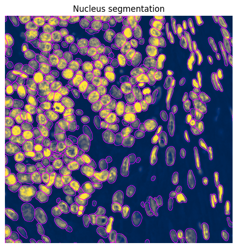
3. Segmentation

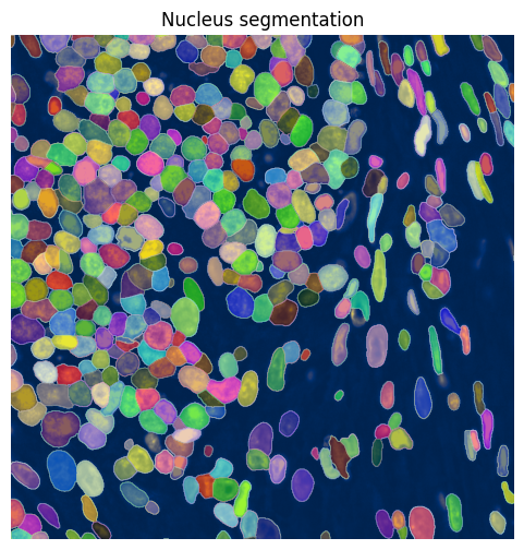
3.1 Nucleus segmentation

To segment the nuclei, we will show an example using Cellpose 3, a deep learning network based on a UNET architecture. Note that we need to make sure that we installed the correct version of Cellpose to use Cellpose 3 and not the newer Cellpose 4. Cellpose 4 (a.k.a. Cellpose-SAM) works really well, but is a lot slower. Unfortunately, we can not simply install the latest version and select which model we want to use using the API.

Multiple parameters need to be given as an input to the cellpose algorithm. We recommend tuning these to achieve optimal segmentation quality (see https://cellpose.readthedocs.io/en/v3.1.1.1/settings.html). It is often a good idea to fine-tune the parameters on a crop of the image (especially when you only have CPU to work with).

• diameter: Includes an estimate of the average nucleus diameter and needs to be given in pixels. If set to None, cellpose will try to estimate the diameter, but this might take a long time and is usually far off. As a guideline, you can use approx. 7 micrometer (in this case 33 pixels at 0.2125 micrometer per pixel) for a standard nucleus, but this may vary depending on your specific tissue, sample…

• device: Defines the device you want to work on. If you only have CPU, you can skip this input parameter.

• flow_threshold: Indicates something about the shape of the masks. If you increase it, more masks with less round shapes will be accepted. Usually set between 0.6 and 0.95 (max. is 1). Lower this parameter if you start segmenting artefacts. Increase it if the segmentation misses some non-round cells.

• mask_threshold: Indicates how many of the possible masks are kept. Decreasing the parameter will output more masks. Larger values will output less masks. Usually set between 0 and -6.

• min_size: Indicates the minimum size of a nucleus.

• model_type: If segmenting whole cells instead of nuclei, set this to ‘cyto’. You can do this with and without a nucleus channel. When you want to include a nucleus channel for the segmentation, make sure your image is 3D and that the first channel contains the complete cell staining and the second one the nucleus channel (put the channel parameter to np.array([1,0])).

import cellpose
from loguru import logger

logger.info(f"Below cells were run with Cellpose version {cellpose.version}.")

For best tiled-segmentation performance, rechunk the image on disk first.

For example, rechunk to (4, 4096, 4096), but adjust this to your available memory.

If you are running on GPU or MPS, use the largest chunk size that fits comfortably in device memory.

If you are running on CPU, choose a chunk size that fits comfortably in RAM. As a rule of thumb, the total memory used by the chunks processed concurrently across workers should fit in available RAM, with extra headroom for overlap and intermediate arrays.

Then run hp.im.segment(..., chunks=None) so Harpy uses that on-disk chunking.

from spatialdata.transformations import get_transformation

arr = hp.im.get_dataarray(sdata, element_name="clahe").data.rechunk((4, 4096, 4096))
transformations = get_transformation(sdata.images["clahe"], get_all=True)

se = hp.im.get_dataarray(sdata, element_name="clahe")
c_coords = se.c.data

sdata = hp.im.add_image(
    sdata,
    arr=arr,
    output_image_name="clahe",
    transformations=transformations,  # copy the transformations
    c_coords=c_coords,
    scale_factors=[2, 2, 2, 2],  # save as multiscale
    overwrite=True,
)
sdata["clahe"]

<xarray.DataTree>
Group: /
├── Group: /scale0
│       Dimensions:  (c: 4, y: 10000, x: 10000)
│       Coordinates:
│         * c        (c) <U22 352B 'DAPI' ... 'AlphaSMA_Vimentin'
│         * y        (y) float64 80kB 0.5 1.5 2.5 3.5 ... 9.998e+03 9.998e+03 1e+04
│         * x        (x) float64 80kB 0.5 1.5 2.5 3.5 ... 9.998e+03 9.998e+03 1e+04
│       Data variables:
│           image    (c, y, x) uint16 800MB dask.array<chunksize=(4, 4096, 4096), meta=np.ndarray>
├── Group: /scale1
│       Dimensions:  (c: 4, y: 5000, x: 5000)
│       Coordinates:
│         * c        (c) <U22 352B 'DAPI' ... 'AlphaSMA_Vimentin'
│         * y        (y) float64 40kB 1.0 3.0 5.0 7.0 ... 9.995e+03 9.997e+03 9.999e+03
│         * x        (x) float64 40kB 1.0 3.0 5.0 7.0 ... 9.995e+03 9.997e+03 9.999e+03
│       Data variables:
│           image    (c, y, x) uint16 200MB dask.array<chunksize=(4, 4096, 4096), meta=np.ndarray>
├── Group: /scale2
│       Dimensions:  (c: 4, y: 2500, x: 2500)
│       Coordinates:
│         * c        (c) <U22 352B 'DAPI' ... 'AlphaSMA_Vimentin'
│         * y        (y) float64 20kB 2.0 6.0 10.0 14.0 ... 9.99e+03 9.994e+03 9.998e+03
│         * x        (x) float64 20kB 2.0 6.0 10.0 14.0 ... 9.99e+03 9.994e+03 9.998e+03
│       Data variables:
│           image    (c, y, x) uint16 50MB dask.array<chunksize=(4, 2500, 2500), meta=np.ndarray>
├── Group: /scale3
│       Dimensions:  (c: 4, y: 1250, x: 1250)
│       Coordinates:
│         * c        (c) <U22 352B 'DAPI' ... 'AlphaSMA_Vimentin'
│         * y        (y) float64 10kB 4.0 12.0 20.0 ... 9.98e+03 9.988e+03 9.996e+03
│         * x        (x) float64 10kB 4.0 12.0 20.0 ... 9.98e+03 9.988e+03 9.996e+03
│       Data variables:
│           image    (c, y, x) uint16 12MB dask.array<chunksize=(4, 1250, 1250), meta=np.ndarray>
└── Group: /scale4
        Dimensions:  (c: 4, y: 625, x: 625)
        Coordinates:
          * c        (c) <U22 352B 'DAPI' ... 'AlphaSMA_Vimentin'
          * y        (y) float64 5kB 8.0 24.0 40.0 56.0 ... 9.96e+03 9.976e+03 9.992e+03
          * x        (x) float64 5kB 8.0 24.0 40.0 56.0 ... 9.96e+03 9.976e+03 9.992e+03
        Data variables:
            image    (c, y, x) uint16 3MB dask.array<chunksize=(4, 625, 625), meta=np.ndarray>

xarray.DataTree

• /scale0(4)

  • Dimensions:
    • c: 4
    • y: 10000
    • x: 10000
  • Coordinates: (3)
    • c
      (c)
      <U22
      'DAPI' ... 'AlphaSMA_Vimentin'

      array(['DAPI', 'ATP1A1_CD45_E-Cadherin', '18S', 'AlphaSMA_Vimentin'],dtype='<U22')

    • y
      (y)
      float64
      0.5 1.5 2.5 ... 9.998e+03 1e+04

      array([5.0000e-01, 1.5000e+00, 2.5000e+00, ..., 9.9975e+03, 9.9985e+03,9.9995e+03])

    • x
      (x)
      float64
      0.5 1.5 2.5 ... 9.998e+03 1e+04

      array([5.0000e-01, 1.5000e+00, 2.5000e+00, ..., 9.9975e+03, 9.9985e+03,9.9995e+03])

  • Data variables: (1)
    • image
      (c, y, x)
      uint16
      dask.array<chunksize=(4, 4096, 4096), meta=np.ndarray>

      transform :

      {'global': SequenceTranslation (c, y, x)[ 0. 18000. 10000.]Identity , 'global_micron': SequenceTranslation (c, y, x)[ 0. 18000. 10000.]SequenceIdentityScale (c, y, x)[1. 0.2125 0.2125]}

      Array Chunk Bytes 762.94 MiB 128.00 MiB Shape (4, 10000, 10000) (4, 4096, 4096) Dask graph 9 chunks in 2 graph layers Data type uint16 numpy.ndarray

  /scale1(4)

  • Dimensions:
    • c: 4
    • y: 5000
    • x: 5000
  • Coordinates: (3)
    • c
      (c)
      <U22
      'DAPI' ... 'AlphaSMA_Vimentin'

      array(['DAPI', 'ATP1A1_CD45_E-Cadherin', '18S', 'AlphaSMA_Vimentin'],dtype='<U22')

    • y
      (y)
      float64
      1.0 3.0 5.0 ... 9.997e+03 9.999e+03

      array([1.000e+00, 3.000e+00, 5.000e+00, ..., 9.995e+03, 9.997e+03, 9.999e+03])

    • x
      (x)
      float64
      1.0 3.0 5.0 ... 9.997e+03 9.999e+03

      array([1.000e+00, 3.000e+00, 5.000e+00, ..., 9.995e+03, 9.997e+03, 9.999e+03])

  • Data variables: (1)
    • image
      (c, y, x)
      uint16
      dask.array<chunksize=(4, 4096, 4096), meta=np.ndarray>

      transform :

      {'global': SequenceScale (y, x)[2. 2.]SequenceTranslation (c, y, x)[ 0. 18000. 10000.]Identity , 'global_micron': SequenceScale (y, x)[2. 2.]SequenceTranslation (c, y, x)[ 0. 18000. 10000.]SequenceIdentityScale (c, y, x)[1. 0.2125 0.2125]}

      Array Chunk Bytes 190.73 MiB 128.00 MiB Shape (4, 5000, 5000) (4, 4096, 4096) Dask graph 4 chunks in 2 graph layers Data type uint16 numpy.ndarray

  /scale2(4)

  • Dimensions:
    • c: 4
    • y: 2500
    • x: 2500
  • Coordinates: (3)
    • c
      (c)
      <U22
      'DAPI' ... 'AlphaSMA_Vimentin'

      array(['DAPI', 'ATP1A1_CD45_E-Cadherin', '18S', 'AlphaSMA_Vimentin'],dtype='<U22')

    • y
      (y)
      float64
      2.0 6.0 ... 9.994e+03 9.998e+03

      array([2.000e+00, 6.000e+00, 1.000e+01, ..., 9.990e+03, 9.994e+03, 9.998e+03])

    • x
      (x)
      float64
      2.0 6.0 ... 9.994e+03 9.998e+03

      array([2.000e+00, 6.000e+00, 1.000e+01, ..., 9.990e+03, 9.994e+03, 9.998e+03])

  • Data variables: (1)
    • image
      (c, y, x)
      uint16
      dask.array<chunksize=(4, 2500, 2500), meta=np.ndarray>

      transform :

      {'global': SequenceScale (y, x)[4. 4.]SequenceTranslation (c, y, x)[ 0. 18000. 10000.]Identity , 'global_micron': SequenceScale (y, x)[4. 4.]SequenceTranslation (c, y, x)[ 0. 18000. 10000.]SequenceIdentityScale (c, y, x)[1. 0.2125 0.2125]}

      Array Chunk Bytes 47.68 MiB 47.68 MiB Shape (4, 2500, 2500) (4, 2500, 2500) Dask graph 1 chunks in 2 graph layers Data type uint16 numpy.ndarray

  /scale3(4)

  • Dimensions:
    • c: 4
    • y: 1250
    • x: 1250
  • Coordinates: (3)
    • c
      (c)
      <U22
      'DAPI' ... 'AlphaSMA_Vimentin'

      array(['DAPI', 'ATP1A1_CD45_E-Cadherin', '18S', 'AlphaSMA_Vimentin'],dtype='<U22')

    • y
      (y)
      float64
      4.0 12.0 ... 9.988e+03 9.996e+03

      array([4.000e+00, 1.200e+01, 2.000e+01, ..., 9.980e+03, 9.988e+03, 9.996e+03])

    • x
      (x)
      float64
      4.0 12.0 ... 9.988e+03 9.996e+03

      array([4.000e+00, 1.200e+01, 2.000e+01, ..., 9.980e+03, 9.988e+03, 9.996e+03])

  • Data variables: (1)
    • image
      (c, y, x)
      uint16
      dask.array<chunksize=(4, 1250, 1250), meta=np.ndarray>

      transform :

      {'global': SequenceScale (y, x)[8. 8.]SequenceTranslation (c, y, x)[ 0. 18000. 10000.]Identity , 'global_micron': SequenceScale (y, x)[8. 8.]SequenceTranslation (c, y, x)[ 0. 18000. 10000.]SequenceIdentityScale (c, y, x)[1. 0.2125 0.2125]}

      Array Chunk Bytes 11.92 MiB 11.92 MiB Shape (4, 1250, 1250) (4, 1250, 1250) Dask graph 1 chunks in 2 graph layers Data type uint16 numpy.ndarray

  /scale4(4)

  • Dimensions:
    • c: 4
    • y: 625
    • x: 625
  • Coordinates: (3)
    • c
      (c)
      <U22
      'DAPI' ... 'AlphaSMA_Vimentin'

      array(['DAPI', 'ATP1A1_CD45_E-Cadherin', '18S', 'AlphaSMA_Vimentin'],dtype='<U22')

    • y
      (y)
      float64
      8.0 24.0 ... 9.976e+03 9.992e+03

      array([8.000e+00, 2.400e+01, 4.000e+01, ..., 9.960e+03, 9.976e+03, 9.992e+03])

    • x
      (x)
      float64
      8.0 24.0 ... 9.976e+03 9.992e+03

      array([8.000e+00, 2.400e+01, 4.000e+01, ..., 9.960e+03, 9.976e+03, 9.992e+03])

  • Data variables: (1)
    • image
      (c, y, x)
      uint16
      dask.array<chunksize=(4, 625, 625), meta=np.ndarray>

      transform :

      {'global': SequenceScale (y, x)[16. 16.]SequenceTranslation (c, y, x)[ 0. 18000. 10000.]Identity , 'global_micron': SequenceScale (y, x)[16. 16.]SequenceTranslation (c, y, x)[ 0. 18000. 10000.]SequenceIdentityScale (c, y, x)[1. 0.2125 0.2125]}

      Array Chunk Bytes 2.98 MiB 2.98 MiB Shape (4, 625, 625) (4, 625, 625) Dask graph 1 chunks in 2 graph layers Data type uint16 numpy.ndarray

import os

import torch
from dask.distributed import Client, LocalCluster
from loguru import logger

"""
We set up a local Dask distributed cluster to overwrite dask default behaviour (threaded processing).
Once the cluster is created, a Dask Client is used to connect to it.
The Dask dashboard link allows you to monitor cluster performance and task progress.
"""

if torch.cuda.is_available():
    device = "cuda"
elif torch.backends.mps.is_available():
    device = "mps"
else:
    device = "cpu"

logger.info(f"Using device: {device}")

n_workers = 1 if device in {"cuda", "mps"} else 12

# Create a local Dask cluster
cluster = LocalCluster(
    n_workers=n_workers,  # Use a single worker for GPU/MPS; otherwise use 12 CPU workers.
    threads_per_worker=1,  # Number of threads per worker
    memory_limit="32GB",  # Memory limit per worker
    local_directory=os.environ.get("TMPDIR"),
)

client = Client(cluster)
logger.info(client.dashboard_link)

# Perform nucleus segmentation
sdata = hp.im.segment(
    sdata,
    image_name="clahe",  # The image element in sdata to be segmented.
    chunks=None,  # Settings chunks=None is equivalent to settings chunks=4096, as chunks on disk are 4096
    depth=200,
    model=hp.im.cellpose_callable,
    # parameters that will be passed to the callable _cellpose:
    pretrained_model="nuclei",  # can also be "cyto", "cyto3", or a path to a fine-tuned cellpose model.
    device=device,
    diameter=33,
    flow_threshold=0.9,
    cellprob_threshold=-4,
    output_labels_name="nucleus_segmentation_mask",
    output_shapes_name="nucleus_segmentation_mask_boundaries",
    crd=None,  # region to segment [x_min, xmax, y_min, y_max], set to [10000,11000,18000,19000] if working on a low end laptop.
    channels=[1, 0],  # This specifies we are segmenting nuclei in grayscale
    overwrite=True,
)

client.close()

# Plot nucleus segmentation results from Cellpose
min_x = 10000
max_x = 11000
min_y = 18000
max_y = 19000

norm = Normalize(vmax=5000, clip=False)

shapes_name = "nucleus_segmentation_mask_boundaries"

# subset first, because we do not want to query the points
sdata_crop = sdata.subset(element_names=["clahe", shapes_name])

sdata_crop = sdata_crop.query.bounding_box(
    min_coordinate=[min_x, min_y],
    max_coordinate=[max_x, max_y],
    axes=("x", "y"),
    target_coordinate_system="global",
)

fig, ax = plt.subplots(1, 1, figsize=(6, 6))

ax = (
    sdata_crop.pl.render_images(
        element="clahe",
        cmap="cividis",
        channel="DAPI",
        norm=norm,
    )
    .pl.render_shapes(
        element=shapes_name,
        fill_alpha=0,
        outline_width=0.5,
        outline_alpha=1,
        outline_color="magenta",
    )
    .pl.show(
        title="Nucleus segmentation",
        coordinate_systems="global",
        colorbar=False,
        ax=ax,
        return_ax=True,
    )
)

ax.set_xlim(min_x, max_x)
ax.set_ylim(min_y, max_y)
ax.invert_yaxis()
ax.axis("off")

(np.float64(10000.0),
 np.float64(11000.0),
 np.float64(19000.0),
 np.float64(18000.0))

Or use the wrapper function harpy.pl.plot_sdata to plot the segmentation mask.

fig, ax = plt.subplots(1, 1, figsize=(6, 6))

channel = "DAPI"

norm = Normalize(vmax=5000, clip=False)

render_labels_kwargs = {"fill_alpha": 0.4, "outline_alpha": 0.5}
render_images_kwargs = {"cmap": "cividis", "norm": norm}

ax = hp.pl.plot_sdata(
    sdata,
    image_name="clahe",
    labels_name="nucleus_segmentation_mask",
    channel=channel,
    crd=(10000, 11000, 18000, 19000),
    to_coordinate_system="global",
    render_images_kwargs=render_images_kwargs,
    render_labels_kwargs=render_labels_kwargs,
    show_kwargs={"title": "Nucleus segmentation", "colorbar": False},
    ax=ax,
)
ax.axis("off")

(np.float64(10000.0),
 np.float64(11000.0),
 np.float64(19000.0),
 np.float64(18000.0))

from spatialdata.transformations import get_transformation

display(
    get_transformation(sdata["nucleus_segmentation_mask"], get_all=True)
)  # -> microns per pixel is 0.2125
microns_per_pixel = 0.2125

{'global': Sequence 
     Translation (y, x)
         [18000. 10000.]
     Identity ,
 'global_micron': Sequence 
     Translation (y, x)
         [18000. 10000.]
     Sequence 
         Identity 
         Scale (y, x)
             [0.2125 0.2125]}

df = hp.qc.segmentation_coverage(
    sdata,
    labels_name="nucleus_segmentation_mask",
    microns_per_pixel=microns_per_pixel,
)
display(df)
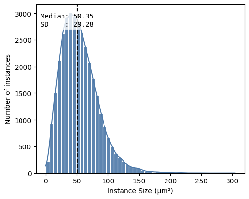
hp.qc.segmentation_histogram(
    sdata,
    labels_name="nucleus_segmentation_mask",
    microns_per_pixel=microns_per_pixel,
    bins=50,
)

	labels_name	total_instances	total_area_μm²	covered_area_μm²	covered_area_percentage
0	nucleus_segmentation_mask	34157	4515625.0	1.856609e+06	41.115214

<Axes: xlabel='Instance Size (μm²)', ylabel='Number of instances'>

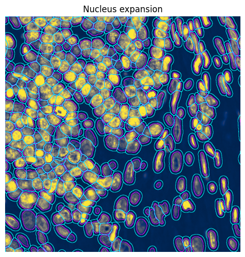
3.2 Nucleus expansion

In some cases, it may be useful to expand de nuclei segmentations to approximate the cell bodies. Note that this is not very precise and, while it increases the number of transcripts assigned to a cell, it also introduces more wrongly assigned transcripts (i.e. that actually belong to other cells).

# Expand labels element masks
sdata = hp.im.expand_labels(
    sdata,
    labels_name="nucleus_segmentation_mask",
    distance=10,  # Number of pixels to expand
    output_labels_name="nucleus_segmentation_mask_expanded",  # Creates a new labels element
    output_shapes_name="nucleus_segmentation_mask_expanded_boundaries",  # Creates a new shapes element
    overwrite=True,
)

min_x = 10000
max_x = 11000
min_y = 18000
max_y = 19000

shapes_name = "nucleus_segmentation_mask_boundaries"
shapes_name_expanded = "nucleus_segmentation_mask_expanded_boundaries"

norm = Normalize(vmax=5000, clip=False)

sdata_crop = sdata.subset(element_names=["clahe", shapes_name, shapes_name_expanded])

sdata_crop = sdata_crop.query.bounding_box(
    min_coordinate=[min_x, min_y],
    max_coordinate=[max_x, max_y],
    axes=("x", "y"),
    target_coordinate_system="global",
)

fig, ax = plt.subplots(figsize=(6, 6))

sdata_crop.pl.render_images(
    element="clahe",
    cmap="cividis",
    channel="DAPI",
    norm=norm,
).pl.render_shapes(
    element="nucleus_segmentation_mask_boundaries",
    fill_alpha=0,
    outline_width=0.5,
    outline_alpha=1,
    outline_color="magenta",
).pl.render_shapes(
    element="nucleus_segmentation_mask_expanded_boundaries",
    fill_alpha=0,
    outline_width=0.5,
    outline_alpha=1,
    outline_color="cyan",
).pl.show(
    title="Nucleus expansion",
    coordinate_systems="global",
    colorbar=False,
    ax=ax,
)

ax.set_xlim(min_x, max_x)
ax.set_ylim(min_y, max_y)
ax.invert_yaxis()
ax.axis("off")

(np.float64(10000.0),
 np.float64(11000.0),
 np.float64(19000.0),
 np.float64(18000.0))

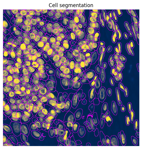
3.3 Cell segmentation

se = hp.im.get_dataarray(sdata, element_name="clahe")
channels_idx = [
    se.c.data.tolist().index("ATP1A1_CD45_E-Cadherin") + 1,
    se.c.data.tolist().index("DAPI") + 1,
]  #  + 1 because CellPose channel specifications are 1-indexed!

channels_idx  # [membrane stain index + 1, nuclear stain index + 1]

[2, 1]

device = "cpu"

sdata = hp.im.segment(
    sdata,
    image_name="clahe",
    chunks=None,
    depth=200,
    model=hp.im.cellpose_callable,
    # parameters that will be passed to the callable _cellpose
    pretrained_model="cyto3",
    device=device,
    diameter=33,
    flow_threshold=0.9,
    cellprob_threshold=-4,
    channels=channels_idx,  # NOTE: channels is deprecated in cellpose 4. Cellpose 4 models will segment on the 'first' three channels by default.
    output_labels_name="cell_segmentation_mask",
    output_shapes_name="cell_segmentation_mask_boundaries",
    crd=[
        10000,
        11000,
        18000,
        19000,
    ],  # region to segment [x_min, xmax, y_min, y_max], we only have one chunk, so we do not use a dask client.
    overwrite=True,
)

# Plot cell segmentation results from Cellpose
min_x = 10000
max_x = 11000
min_y = 18000
max_y = 19000

norm = Normalize(vmax=5000, clip=False)

shapes_name = "cell_segmentation_mask_boundaries"

# subset first, because we do not want to query the points
sdata_crop = sdata.subset(element_names=["clahe", shapes_name])

sdata_crop = sdata_crop.query.bounding_box(
    min_coordinate=[min_x, min_y],
    max_coordinate=[max_x, max_y],
    axes=("x", "y"),
    target_coordinate_system="global",
)

fig, ax = plt.subplots(1, 1, figsize=(6, 6))

ax = (
    sdata_crop.pl.render_images(
        element="clahe",
        cmap="cividis",
        channel="DAPI",
        norm=norm,
    )
    .pl.render_shapes(
        element=shapes_name,
        fill_alpha=0,
        outline_width=0.5,
        outline_alpha=1,
        outline_color="magenta",
    )
    .pl.show(
        title="Cell segmentation",
        coordinate_systems="global",
        colorbar=False,
        ax=ax,
        return_ax=True,
    )
)

ax.set_xlim(min_x, max_x)
ax.set_ylim(min_y, max_y)
ax.invert_yaxis()
ax.axis("off")

(np.float64(10000.0),
 np.float64(11000.0),
 np.float64(19000.0),
 np.float64(18000.0))

4. Create the AnnData table

4.1 Creating the count matrix

The transcripts were already read into the SpatialData by the Xenium reader function. For some spatial technologies, it might be necessary to use the general harpy.io.read_transcripts function, which you can configure for most types of transcript data. There are also specific reader functions for Resolve Biosciences Molecular Cartography data (harpy.io.read_resolve_transcripts) and for Vizgen Merscope data (harpy.io.read_merscope_transcripts).

Once the transcripts are read in and we have a segmentation mask, we can allocate the transcripts to the correct cell. This allocation step creates the count matrix saved in an AnnData object.

# Inspect the points element
sdata.points["transcripts_global"].head()

	x	y	gene
0	18908.382353	27736.764706	AAMP
0	18180.441176	27247.500000	A2ML1
0	13668.970588	27754.044118	A2ML1
0	15351.176471	27958.235294	AAMP
0	17088.161765	27187.058824	AAMP

from spatialdata.transformations import get_transformation

get_transformation(sdata.points["transcripts_global"], get_all=True)

{'global': Identity ,
 'global_micron': Affine (x, y -> x, y)
     [0.2125 0.     0.    ]
     [0.     0.2125 0.    ]
     [0. 0. 1.]}

# Allocate transcripts to cells based on the segmentation masks
sdata = hp.tb.allocate(
    sdata=sdata,
    labels_name="nucleus_segmentation_mask",  # The labels element (i.e. nucleus_segmentation mask) in `sdata` to be used to allocate the transcripts to cells.
    points_name="transcripts_global",  # The points element in `sdata` that contains the transcripts.
    output_table_name="table_transcriptomics",  # The table element in `sdata` in which to save the AnnData object with the transcripts counts per cell.
    to_coordinate_system="global",  # NOTE: always run the allocation step in the pixel coordinate system. Relation between the points element and this coordinate system should be an Identity.
    update_shapes_elements=False,
    overwrite=True,
)

# Inspect the SpatialData metadata stored in `.uns`.
#
# `hp.tb.allocate(...)` does not only create an AnnData count matrix, it also annotates the
# table so that SpatialData and Harpy know how each table row maps back to the segmentation.
# This metadata lives in `adata.uns[TableModel.ATTRS_KEY]`.
#
# In particular:
# - `TableModel.INSTANCE_KEY` gives the name of the `.obs` column holding the instance ids
#   (for example `cell_ID`).
# - `TableModel.REGION_KEY_KEY` gives the name of the `.obs` column holding the region or
#   labels-layer assignment for each row.
# - `TableModel.REGION_KEY` gives the labels element(s) in `sdata` that this table annotates.
#
# Together, these fields tell Harpy which segmentation layer to use and which label id within
# that layer corresponds to each row. This is what allows downstream functions and plotting
# utilities to keep the AnnData table synchronized with the SpatialData object.
from spatialdata.models import TableModel

table = sdata.tables["table_transcriptomics"]

# Inspect the new table element.
display(table)

logger.info(
    f"Number of cells: {len(table.obs.index)}",
)
logger.info(
    f"Number of genes: {len(table.var.index)}",
)

# Full SpatialData annotation metadata for this table.
logger.info(table.uns[TableModel.ATTRS_KEY])

# Name of the `.obs` column that stores the region or labels-layer assignment.
logger.info(table.uns[TableModel.ATTRS_KEY][TableModel.REGION_KEY_KEY])

# Name of the `.obs` column that stores the instance ids.
logger.info(table.uns[TableModel.ATTRS_KEY][TableModel.INSTANCE_KEY])

# Labels layer(s) in `sdata` that are annotated by this table.
logger.info(table.uns[TableModel.ATTRS_KEY][TableModel.REGION_KEY])

# The corresponding columns can be inspected directly in `.obs`.
display(table.obs.head())

AnnData object with n_obs × n_vars = 34121 × 5100
    obs: 'cell_ID', 'fov_labels'
    uns: 'spatialdata_attrs'
    obsm: 'spatial'

	cell_ID	fov_labels
cells
1080_nucleus_segmentation_mask_ca701a09	1080	nucleus_segmentation_mask
1128_nucleus_segmentation_mask_ca701a09	1128	nucleus_segmentation_mask
1192_nucleus_segmentation_mask_ca701a09	1192	nucleus_segmentation_mask
1208_nucleus_segmentation_mask_ca701a09	1208	nucleus_segmentation_mask
1256_nucleus_segmentation_mask_ca701a09	1256	nucleus_segmentation_mask

# Inspect the spatial coordinates stored in obsm
sdata.tables["table_transcriptomics"].obsm["spatial"][
    :5
]  # x,y,(z) coordinates of cell centroid (calculated based on mean transcripts location)

array([[19240.93661972, 26164.88028169],
       [18523.41935484, 26173.17741935],
       [18556.78947368, 26190.98245614],
       [18877.        , 26188.33333333],
       [18705.4       , 26193.13333333]])

4.2 Support for spatial proteomics

hp.tb.allocate_intensity(...) aggregates image intensities over segmented objects and stores the result as an AnnData table in sdata.tables. In other words, it converts a raster image element together with a labels element into a per-cell feature table, where each row corresponds to one segmented object and each column corresponds to one image channel.

This is especially useful for proteomics workflows, where multi-channel images encode marker intensities rather than transcript counts. Depending on the selected mode, Harpy can compute, for example, the mean or summed intensity per cell per channel, and it can also add additional summary statistics to .obs.

Importantly, this workflow is designed to scale to very large images. Harpy processes the image in chunks using Dask, so intensity extraction remains feasible for large multiplexed datasets that do not fit into memory as a single array. When working with backed SpatialData objects, it is often best to keep chunks=None and rely on well-chosen on-disk chunking.

sdata = hp.tb.allocate_intensity(
    sdata,
    image_name="morphology_focus_global",
    labels_name="nucleus_segmentation_mask",
    output_table_name="table_proteomics",
    mode="mean",
    obs_stats="var",
    calculate_center_of_mass=True,
)

display(sdata["table_proteomics"].to_df().head())
display(sdata["table_proteomics"].obs.head())

channels	DAPI	ATP1A1_CD45_E-Cadherin	18S	AlphaSMA_Vimentin
cells
1080_nucleus_segmentation_mask_39d08691	981.235168	307.473724	115.444069	162.813553
1128_nucleus_segmentation_mask_39d08691	1304.929321	228.890167	106.314941	134.339020
1192_nucleus_segmentation_mask_39d08691	1432.931274	653.448486	74.252861	359.208801
1208_nucleus_segmentation_mask_39d08691	550.600464	264.447937	10.476997	55.566586
1240_nucleus_segmentation_mask_39d08691	236.990524	366.909943	21.028437	267.127960

	cell_ID	fov_labels	var_DAPI	var_ATP1A1_CD45_E-Cadherin	var_18S	var_AlphaSMA_Vimentin
cells
1080_nucleus_segmentation_mask_39d08691	1080	nucleus_segmentation_mask	219549.796875	27741.378906	3862.941162	25551.103516
1128_nucleus_segmentation_mask_39d08691	1128	nucleus_segmentation_mask	397282.468750	6039.265137	4853.724121	2873.881836
1192_nucleus_segmentation_mask_39d08691	1192	nucleus_segmentation_mask	760799.625000	19651.898438	1032.331665	39414.433594
1208_nucleus_segmentation_mask_39d08691	1208	nucleus_segmentation_mask	125082.570312	7182.421387	26.031553	2531.504639
1240_nucleus_segmentation_mask_39d08691	1240	nucleus_segmentation_mask	10627.659180	5972.593750	50.103455	3363.998047

# Inspect the spatial coordinates stored in obsm
sdata.tables["table_proteomics"].obsm["spatial"][
    :5
]  # x,y,(z) coordinates of nucleus centroid (center of mass of each nucleus)

array([[19228.        , 26168.04449153],
       [18517.35456369, 26174.82898696],
       [18557.93656388, 26189.91365639],
       [18883.93220339, 26191.67312349],
       [18846.11374408, 26190.57345972]])

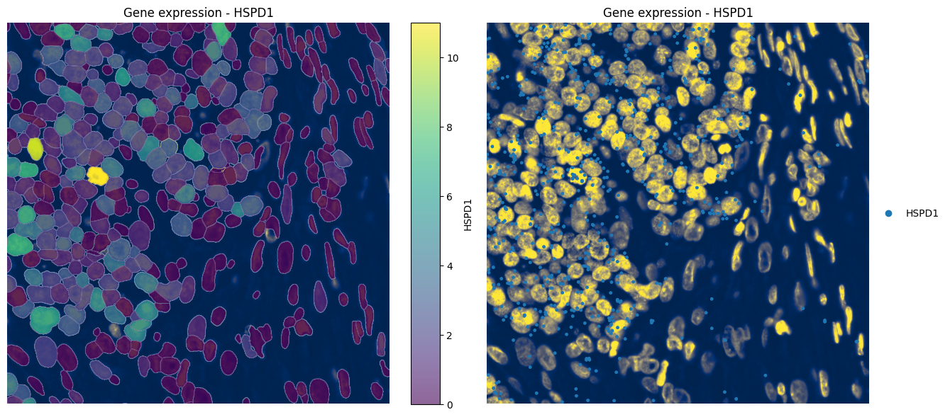
4.3 Visualizing gene expression

fig, axes = plt.subplots(1, 2, figsize=(16, 7))

channel = "DAPI"

norm = Normalize(vmax=5000, clip=False)

render_labels_kwargs = {"fill_alpha": 0.6, "outline_alpha": 0.5}
render_images_kwargs = {"cmap": "cividis", "norm": norm, "colorbar": False}

_ax = hp.pl.plot_sdata(
    sdata,
    image_name="clahe",
    labels_name="nucleus_segmentation_mask",
    table_name="table_transcriptomics",
    color="HSPD1",
    channel=channel,
    crd=(10000, 11000, 18000, 19000),
    to_coordinate_system="global",
    render_images_kwargs=render_images_kwargs,
    render_labels_kwargs=render_labels_kwargs,
    show_kwargs={"title": "Gene expression - HSPD1", "colorbar": True},
    ax=axes[0],
)
_ax.axis("off")


_ax = hp.pl.plot_sdata_genes(
    sdata,
    image_name="clahe",
    points_name="transcripts_global",
    genes="HSPD1",
    channel=channel,
    crd=(10000, 11000, 18000, 19000),
    to_coordinate_system="global",
    render_images_kwargs=render_images_kwargs,
    show_kwargs={"title": "Gene expression - HSPD1", "colorbar": True},
    ax=axes[1],
)
_ax.axis("off")

(np.float64(10000.0),
 np.float64(11000.0),
 np.float64(19000.0),
 np.float64(18000.0))

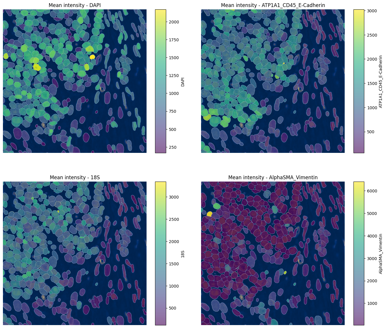
4.4 Visualizing mean intensity

channels = hp.im.get_dataarray(sdata, element_name="morphology_focus_global").c.data
channels

array(['DAPI', 'ATP1A1_CD45_E-Cadherin', '18S', 'AlphaSMA_Vimentin'],
      dtype='<U22')

fig, axes = plt.subplots(2, 2, figsize=(16, 14))
axes = axes.flatten()

channel = "DAPI"

norm = Normalize(vmax=5000, clip=False)

render_labels_kwargs = {"fill_alpha": 0.6, "outline_alpha": 0.5}
render_images_kwargs = {"cmap": "cividis", "norm": norm, "colorbar": False}

for ax, color in zip(axes, channels, strict=True):
    _ax = hp.pl.plot_sdata(
        sdata,
        image_name="clahe",
        labels_name="nucleus_segmentation_mask",
        table_name="table_proteomics",
        color=color,
        channel=channel,
        crd=(10000, 11000, 18000, 19000),
        to_coordinate_system="global",
        render_images_kwargs=render_images_kwargs,
        render_labels_kwargs=render_labels_kwargs,
        show_kwargs={"title": f"Mean intensity - {color}", "colorbar": True},
        ax=ax,
    )
    _ax.axis("off")

# plt.tight_layout()

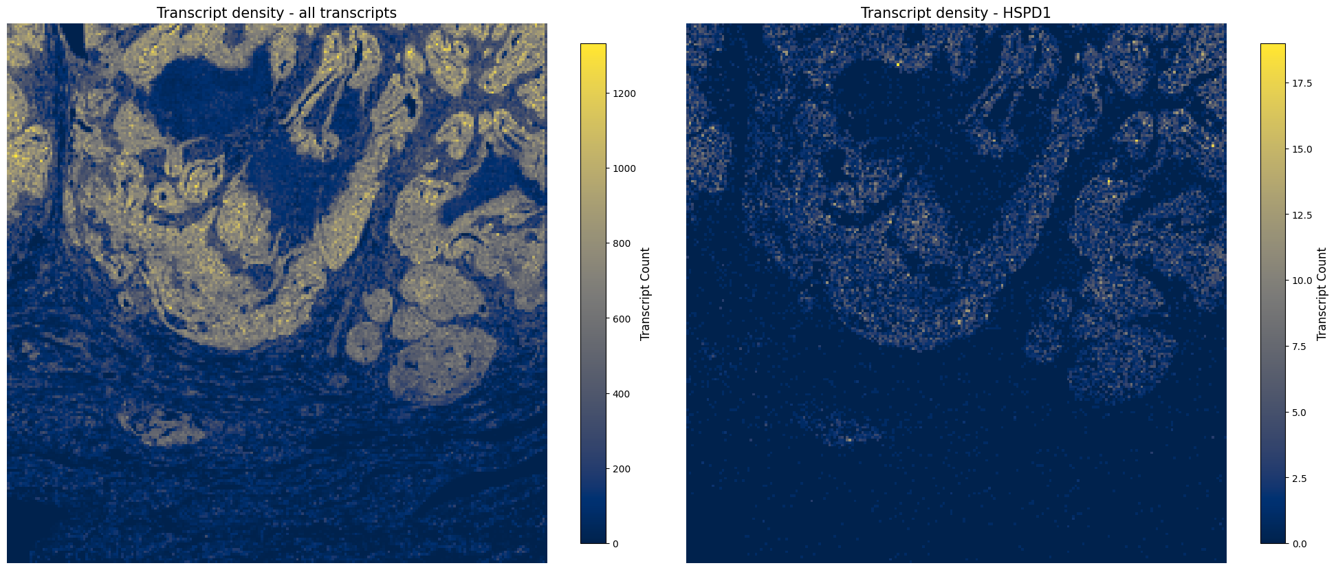
4.5 Transcript quality

After we have created the AnnData object, we want to check transcript quality. We first create transcript density plots directly from the transcript points to assess whether transcript density is similar across the tissue. If this is not the case, there can be multiple biological or technical reasons, and gene panel composition can also have an influence.

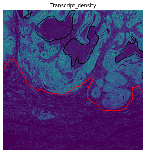
Later, we use hp.im.transcript_density(...) to convert the transcript points into a transcript-density image element. This rasterized layer can then be visualized together with region annotations such as tumor and necrosis.

fig, axes = plt.subplots(1, 2, figsize=(20, 10))

ax = hp.pl.plot_transcript_density(
    sdata,
    bin_size=10,  # bin size in micron if we specify micron coordinate system
    points_name="transcripts_global",
    to_coordinate_system="global_micron",
    cmap="cividis",
    frac=1,
    ax=axes[0],
)
ax.set_title("Transcript density - all transcripts", fontsize=15)
ax.axis("off")

ax = hp.pl.plot_transcript_density(
    sdata,
    bin_size=10,  # bin size in micron if we specify micron coordinate system
    genes="HSPD1",
    cmap="cividis",
    # crd=(10000*0.2125, 11000*0.2125, 18000*0.2125, 19000*0.2125),
    points_name="transcripts_global",
    to_coordinate_system="global_micron",
    frac=1,
    ax=axes[1],
)
ax.set_title("Transcript density - HSPD1", fontsize=15)
ax.axis("off")

plt.tight_layout()

# Create transcript density image
sdata = hp.im.transcript_density(
    sdata,
    image_name="clahe",  # The layer of the SpatialData object used for determining image boundary.
    points_name="transcripts_global",  # The layer name that contains the transcript data points, by default "transcripts".
    output_image_name="transcript_density",  # The name of the output image element
    overwrite=True,
)

# Compare the transcript-density image element against our region annotations for tumor and necrosis
fig, ax = plt.subplots(figsize=(6, 6))

sdata.pl.render_images(
    element="transcript_density",
).pl.render_shapes(
    element="tumor", color="red", fill_alpha=0, outline_alpha=1, outline_color="red"
).pl.render_shapes(
    element="necrosis",
    color="black",
    fill_alpha=0,
    outline_alpha=1,
    outline_color="black",
).pl.show(
    title="Transcript_density",
    coordinate_systems="global",
    colorbar=False,
    ax=ax,
)

ax.set_xlim(10000, 20000)
ax.set_ylim(18000, 28000)
ax.invert_yaxis()
ax.axis("off")

(np.float64(10000.0),
 np.float64(20000.0),
 np.float64(28000.0),
 np.float64(18000.0))

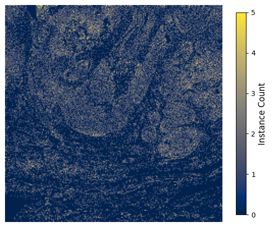
Next, we inspect the nuclei density. This allows us to assess how densely segmented instances are distributed across the tissue and to compare this spatial pattern against the transcript-density signal and the tissue annotations.

fig, ax = plt.subplots(figsize=(7, 7))

hp.pl.plot_instance_density(
    sdata,
    bin_size=10
    / microns_per_pixel,  # bin size in pixels because .obsm["spatial"] is in pixels in our case
    labels_name="nucleus_segmentation_mask",
    table_name="table_transcriptomics",
    spatial_key="spatial",  # we will use the centroids of the nuclei to determine instance density
    ax=ax,
)
ax.axis("off")

(np.float64(10000.0),
 np.float64(20023.52941176489),
 np.float64(28023.52941176489),
 np.float64(18000.0))

# Check number of transcripts
print(
    "Number of transcripts in points element: ", len(sdata.points["transcripts_global"])
)
print(
    "Number of transcripts assigned to cells: ",
    sdata.tables["table_transcriptomics"].X.sum(),
)
print(
    "Percentage of transcripts kept: ",
    (
        (sdata.tables["table_transcriptomics"].X.sum())
        / len(sdata.points["transcripts_global"])
    )
    * 100,
)

# Check number of genes
print(
    "Number of genes in points element: ",
    sdata.points["transcripts_global"].compute()["gene"].nunique(),
)
print(
    "Number of genes found in cells: ",
    len(sdata.tables["table_transcriptomics"].var.index),
)

# Note: In general, we do not want to lose any genes, but this may happen for low-abundance genes.

Number of transcripts in points element:  13028066
Number of transcripts assigned to cells:  9065635
Percentage of transcripts kept:  69.58542426788443
Number of genes in points element:  5101
Number of genes found in cells:  5100

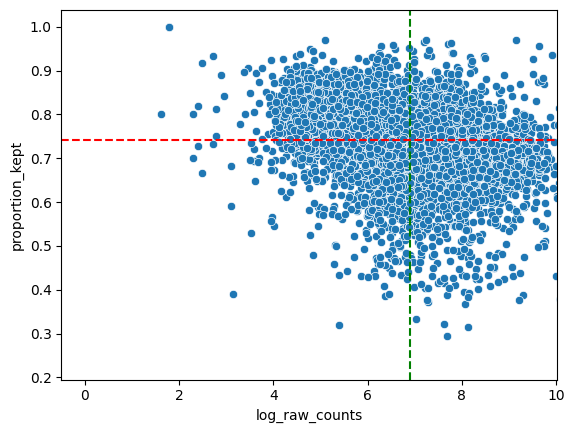
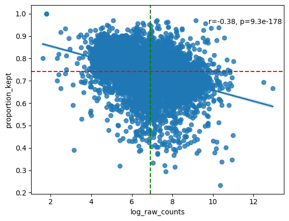
# Analyse and visualize the proportion of transcripts that could not be assigned to a cell during allocation step.
df_analyse_genes_left_out = hp.qc.analyse_genes_left_out(
    sdata,
    labels_name="nucleus_segmentation_mask",
    table_name="table_transcriptomics",
    points_name="transcripts_global",
)

# NOTE: In general we see a downward trend. The more a gene is measured, the less it is located in cells (in ratio).
# NOTE: The function also prints the ten genes with the highest proportion of transcripts filtered out. If a lot of these genes are markers for the same cell type, you will want to find out why this is happening (bad staining, large cell body compared to nucleus, etc.)

# Inspect analyse_genes_left_out() output table
df_analyse_genes_left_out.sort_values(by="proportion_kept", ascending=True)

	proportion_kept	raw_counts	log_raw_counts
MYH11	0.233222	31828	10.368102
SYNPO2	0.293735	2155	7.675546
HOPX	0.314537	3405	8.133000
IGF2	0.319820	222	5.402677
PLN	0.321146	2024	7.612831
...	...	...	...
LENG8	0.968997	9354	9.143559
U2AF1	0.969042	1389	7.236339
CRYBB3	0.969136	162	5.087596
F2	1.000000	6	1.791759
Human_CTNNB1_S33C_ALT:G	1.000000	6	1.791759

5100 rows × 3 columns

5. Processing the AnnData table

Harpy integrates with Scanpy for transcriptomics preprocessing. We provide the convenience wrapper hp.tb.preprocess_transcriptomics(...), which runs the standard preprocessing steps on a table stored in a SpatialData object and writes the result back to sdata.

Here, we show the workflow explicitly instead to illustrate integration with Scanpy. Starting from the transcript counts table, we calculate QC metrics, filter low-count cells and low-abundance genes, store the unprocessed counts in .layers["raw_counts"], and then apply instance size normalization, log1p, and scaling.

# Set up the AnnData object used in the explicit workflow.
import pandas as pd
import scanpy as sc
from spatialdata.models import TableModel
from scipy.sparse import issparse

labels_name = "nucleus_segmentation_mask"
table_name = "table_transcriptomics"
raw_counts_key = "raw_counts"

adata = sdata.tables[table_name].copy()

# Harpy-specific step: add the instance size (`instance_size`) to `.obs` using the segmentation mask.
instance_key = adata.uns[TableModel.ATTRS_KEY][TableModel.INSTANCE_KEY]
region_key = adata.uns[TableModel.ATTRS_KEY][TableModel.REGION_KEY_KEY]
labels = hp.im.get_dataarray(sdata, element_name=labels_name)
shape_size = hp.utils.get_instance_size(
    labels.data[None, ...],
    instance_key=instance_key,
    instance_size_key="instance_size",
)
shape_size[region_key] = labels_name
old_index = adata.obs.index
index_name = adata.obs.index.name or "index"
adata.obs = pd.merge(
    adata.obs.reset_index(),
    shape_size,
    on=[instance_key, region_key],
    how="left",
)
adata.obs.index = old_index
adata.obs = adata.obs.drop(columns=[index_name])

# QC metrics + filtering
sc.pp.calculate_qc_metrics(adata, percent_top=(2, 5), inplace=True)
sc.pp.filter_cells(adata, min_counts=10)
sc.pp.filter_genes(adata, min_cells=5)

# Store the unprocessed counts matrix before normalization / transformation.
adata.layers[raw_counts_key] = adata.X.copy()

# Size normalization, log1p, and scaling.
X_size_norm = (
    adata.X.T * 100 / adata.obs["instance_size"].values
).T  # *100 for numerical stability.
if issparse(adata.X):
    adata.X = X_size_norm.tocsr()
else:
    adata.X = X_size_norm

sc.pp.log1p(adata)
adata.raw = adata.copy()
sc.pp.scale(adata, max_value=10)

We write the resulting AnnData object to a new table slot in the Zarr-backed SpatialData object, rather than overwriting the original table.

This is convenient because preprocessing modifies the count matrix. By keeping the original table unchanged, we can easily rerun preprocessing with different parameters without having to reconstruct a clean AnnData object with raw counts first.

sdata = hp.tb.add_table(
    sdata,
    adata=adata,
    output_table_name="table_transcriptomics_preprocessed",  # we save to a new slot
    region=adata.uns[TableModel.ATTRS_KEY][TableModel.REGION_KEY],
    instance_key=adata.uns[TableModel.ATTRS_KEY][TableModel.INSTANCE_KEY],
    region_key=adata.uns[TableModel.ATTRS_KEY][TableModel.REGION_KEY_KEY],
    overwrite=True,
)

display(sdata.tables["table_transcriptomics_preprocessed"])

AnnData object with n_obs × n_vars = 33503 × 5099
    obs: 'cell_ID', 'fov_labels', 'instance_size', 'n_genes_by_counts', 'log1p_n_genes_by_counts', 'total_counts', 'log1p_total_counts', 'pct_counts_in_top_2_genes', 'pct_counts_in_top_5_genes', 'n_counts'
    var: 'n_cells_by_counts', 'mean_counts', 'log1p_mean_counts', 'pct_dropout_by_counts', 'total_counts', 'log1p_total_counts', 'n_cells', 'mean', 'std'
    uns: 'spatialdata_attrs', 'log1p'
    obsm: 'spatial'
    layers: 'raw_counts'

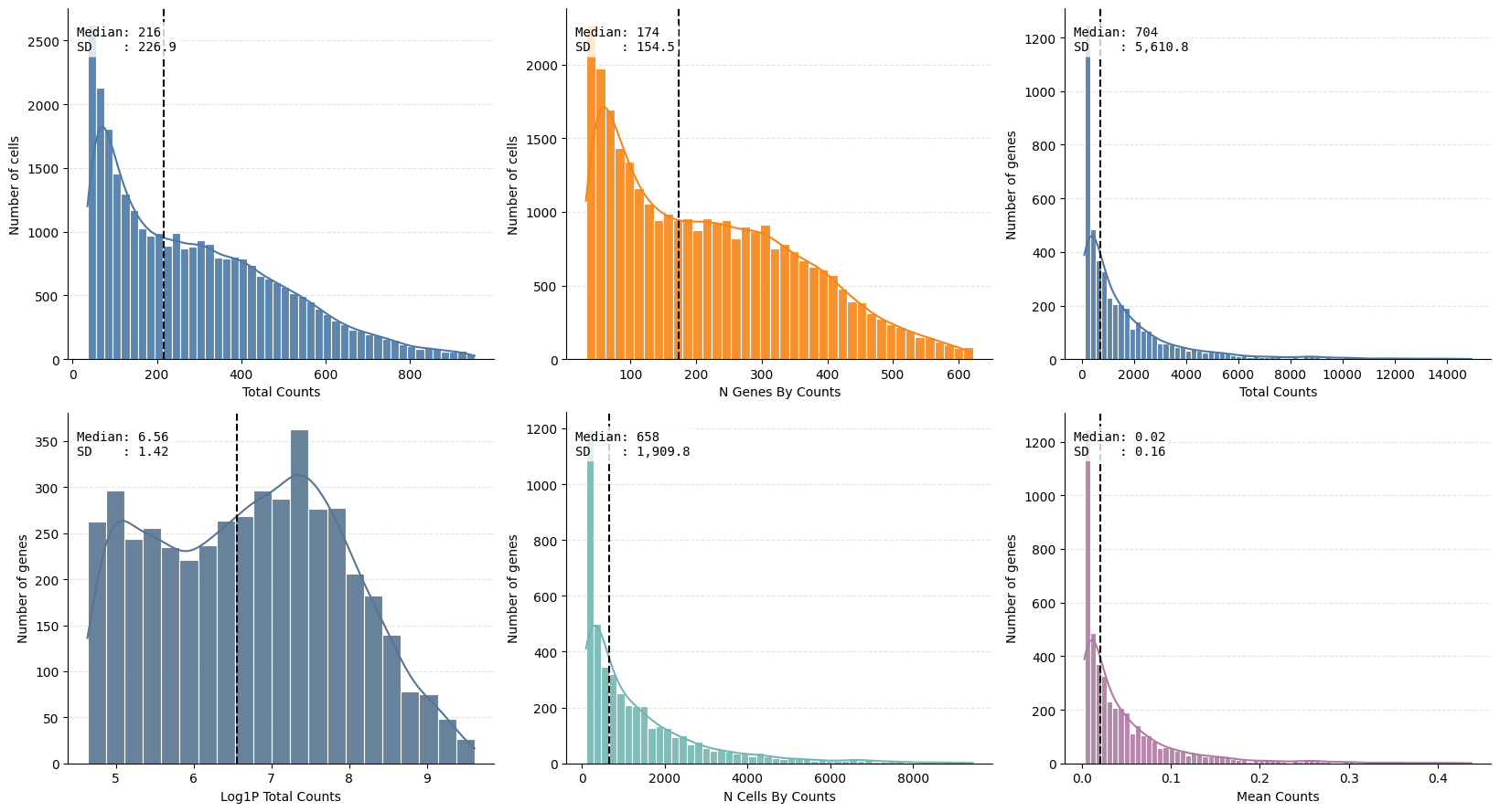
ax = hp.qc.metrics_histogram(
    sdata, table_name="table_transcriptomics_preprocessed", quantile_range=(0.1, 0.99)
)

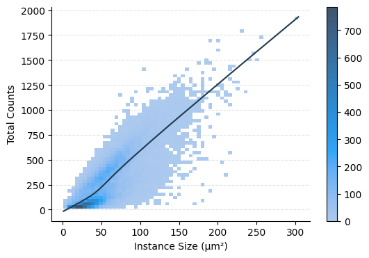
sdata["table_transcriptomics_preprocessed"].obs["instance_size_microns"] = sdata[
    "table_transcriptomics_preprocessed"
].obs["instance_size"] * (microns_per_pixel**2)

ax = hp.qc.obs_scatter(
    sdata,
    table_name="table_transcriptomics_preprocessed",
    column_y="total_counts",
    column_x="instance_size_microns",
    display_column_x="Instance Size (μm²)",
)

Harpy also integrates with Scanpy for clustering. We provide the convenience wrapper hp.tb.leiden(...), which computes the neighborhood graph, optionally calculates a UMAP, runs Leiden clustering, and writes the result back into the SpatialData object.

Here, we again show the workflow explicitly. We first compute PCA on the preprocessed table. We then calculate neighbors, compute a UMAP, run Leiden clustering, rank marker genes per cluster, and finally store the clustered AnnData object in a new table slot.

# Equivalent explicit Scanpy workflow for `hp.tb.leiden(...)`
from spatialdata.models import TableModel

table_name = "table_transcriptomics_preprocessed"
output_table_name = "table_transcriptomics_preprocessed"
key_added = "leiden"
n_comps = 50
n_neighbors = 35
n_pcs = 17
resolution = 0.4
random_state = 100

adata = sdata.tables[table_name].copy()

sc.settings.n_jobs = -1  # use all available CPU cores

# PCA first, because neighbors / UMAP / Leiden are run on the preprocessed representation.
logger.info("Starting PCA")
n_comps = min(n_comps, min(adata.shape) - 1)
sc.pp.pca(adata, n_comps=n_comps)

# Neighborhood graph, UMAP, Leiden clustering, and marker ranking.
logger.info("Starting neighbor graph computation")
sc.pp.neighbors(adata, n_neighbors=n_neighbors, n_pcs=n_pcs, random_state=random_state)
logger.info("Starting UMAP")
sc.tl.umap(adata, random_state=random_state)
logger.info("Starting Leiden clustering")
sc.tl.leiden(
    adata, resolution=resolution, key_added=key_added, random_state=random_state
)
adata.obs[key_added] = adata.obs[key_added].astype(int).astype("category")
logger.info("Starting marker gene ranking")
sc.tl.rank_genes_groups(adata, groupby=key_added, method="wilcoxon")

# Harpy-specific step: write the clustered AnnData object back into the SpatialData object.
logger.info("Writing clustered AnnData object back to SpatialData")
sdata = hp.tb.add_table(
    sdata,
    adata=adata,
    output_table_name=output_table_name,
    region=adata.uns[TableModel.ATTRS_KEY][TableModel.REGION_KEY],
    instance_key=adata.uns[TableModel.ATTRS_KEY][TableModel.INSTANCE_KEY],
    region_key=adata.uns[TableModel.ATTRS_KEY][TableModel.REGION_KEY_KEY],
    overwrite=True,
)

display(sdata.tables[output_table_name])

AnnData object with n_obs × n_vars = 33503 × 5099
    obs: 'cell_ID', 'fov_labels', 'instance_size', 'n_genes_by_counts', 'log1p_n_genes_by_counts', 'total_counts', 'log1p_total_counts', 'pct_counts_in_top_2_genes', 'pct_counts_in_top_5_genes', 'n_counts', 'instance_size_microns', 'leiden'
    var: 'n_cells_by_counts', 'mean_counts', 'log1p_mean_counts', 'pct_dropout_by_counts', 'total_counts', 'log1p_total_counts', 'n_cells', 'mean', 'std'
    uns: 'pca', 'log1p', 'umap', 'spatialdata_attrs', 'leiden', 'rank_genes_groups', 'neighbors'
    obsm: 'X_pca', 'X_umap', 'spatial'
    varm: 'PCs'
    layers: 'raw_counts'
    obsp: 'connectivities', 'distances'

# We can plot other variables on the UMAP as well
from matplotlib.pyplot import rc_context

color_vars = [
    "n_counts",
    "n_genes_by_counts",
    "instance_size",
    "TPX2",
    "leiden",
]
with rc_context({"figure.figsize": (3, 3)}):
    sc.pl.umap(
        sdata.tables["table_transcriptomics_preprocessed"],
        color=color_vars,
        ncols=3,
        frameon=False,
    )

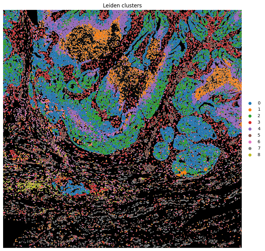
# Plot clusters spatially

fig, ax = plt.subplots(1, 1, figsize=(10, 10))

hp.pl.plot_sdata(
    sdata,
    ax=ax,
    image_name="clahe",
    channel="DAPI",
    table_name="table_transcriptomics_preprocessed",
    labels_name="nucleus_segmentation_mask",
    color="leiden",
    # crd=(min_x, max_x, min_y, max_y),
    to_coordinate_system="global",
    render_images_kwargs={"cmap": "grey"},
    render_labels_kwargs={"fill_alpha": 1},
    show_kwargs={"title": "Leiden clusters", "colorbar": False},
)

ax.axis("off")

(np.float64(10000.0),
 np.float64(20000.0),
 np.float64(28000.0),
 np.float64(18000.0))

6. Cell type annotation

Cell type annotation is fairly complex and requires a lot of biological insights to do correctly. We will show some approaches here, but others exist as well.

10X Genomics has a good analysis guide on how they annotated the cell types in this dataset using label transfer from an accompanying scRNAseq reference dataset.

We have also explored and recreated 10X genomics’ annotation for the full dataset using Harpy. You can find the tutorial here.

6.1 Annotating clusters

# First, we specify a dictionary with marker genes for the different cell types of interest.
marker_genes_dict = {
    "Urothelial-like Cells": [
        "SLC40A1",
        "TRIM29",
        "DSC3",
        "TNS4",
        "PLAT",
        "ANXA8",
        "AVPI1",
        "FGFR3",
    ],
    "Proliferative Tumor Cells": [
        "SMC4",
        "UCHL1",
        "TPX2",
        "BIRC5",
        "TOP2A",
        "STMN1",
        "MYBL2",
        "CENPF",
        "CDK1",
        "TYMS",
    ],
    "Tumor Cells": ["PLXNB1", "CP", "NORAD", "PRKCI", "MUC16", "RGL3"],
    "Tumor Associated Fibroblasts": [
        "LUM",
        "BGN",
        "COL5A1",
        "MMP14",
        "CTHRC1",
        "COL5A2",
        "CCN2",
        "COL11A1",
        "THBS2",
        "LOXL1",
        "CDH11",
        "PLAU",
        "INHBA",
        "SERPINE1",
        "ADAMTS14",
        "LOX",
    ],
    "Smooth Muscle Cells": ["MYH11", "C11orf96", "CNN1"],
    "Macrophages": ["C1QC", "MS4A6A", "AIF1", "FCGR2A", "ITGB2", "CD14", "MSR1"],
    "SOX2-OTpos Tumor Cells": ["NAMPT", "SOST", "SOX2-OT"],
    "Stromal Associated Fibroblasts": ["C7", "ABCA10"],
    "Stromal Associated Endothelial Cells": ["AQP1", "EPAS1"],
    "T and NK Cells": ["TRAC", "CD52", "CD8A", "TRBC1"],
    "Pericytes": ["COL4A1", "HEYL", "PDGFRB", "ENPEP", "AVPR1A", "RGS5", "PDGFA"],
    "Tumor Associated Endothelial Cells": [
        "FLT1",
        "PLVAP",
        "PTPRB",
        "ESM1",
        "CD93",
        "PECAM1",
        "NOTCH4",
        "EGFL7",
        "CLEC14A",
    ],
    "VEGFApos Tumor Cells": [
        "TFPI2",
        "NDRG1",
        "SLC2A1",
        "VEGFA",
        "AMOTL2",
        "P4HA1",
        "ALDOA",
        "ANKRD33B",
    ],
    "Fallopian Tube Epithelium": ["AC007906.2", "KCNC3", "PFKFB3"],
    "Malignant Cells Lining Cyst": [
        "CLDN1",
        "C4B",
        "PROCR",
        "C4A",
        "DSC3",
        "PRG4",
        "RGS4",
        "CALB2",
        "BNC1",
        "CPA4",
    ],
    "Inflammatory Tumor Cells": [
        "MX1",
        "STAT1",
        "IFI44L",
        "SAMD9",
        "IFIT1",
        "PLSCR1",
        "IFIT3",
        "GBP1",
        "DDX58",
        "OAS3",
        "RSAD2",
        "CXCL10",
        "IFIT2",
        "IFI35",
        "PNPT1",
        "IFIH1",
        "OAS1",
        "TNFSF10",
    ],
    "Ciliated Epithelial Cells": [
        "C20orf85",
        "CFAP100",
        "FAM183A",
        "TEKT1",
        "TPPP3",
        "ERICH3",
        "CDHR4",
        "FAM216B",
        "IL5RA",
        "CFAP47",
        "LDLRAD1",
    ],
}

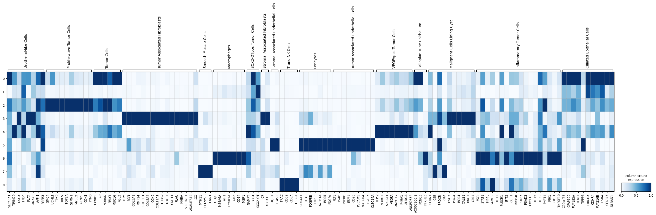
# We can visualize the expression of these marker genes in the Leiden clusters using a scanpy's matrix plot.
import scanpy as sc

sc.pl.matrixplot(
    sdata.tables["table_transcriptomics_preprocessed"],
    var_names=marker_genes_dict,
    groupby="leiden",
    cmap="Blues",
    standard_scale="var",
    colorbar_title="column scaled\nexpression",
    figsize=(32, 6),
)

1.2 Annotating cells using sc.tl.score_genes

We can also use a marker gene list and score cells for each cell type using those markers via scanpy’s sc.tl.score_genes function.

import pandas as pd

all_genes = sorted({gene for genes in marker_genes_dict.values() for gene in genes})

# Create one-hot matrix
df = pd.DataFrame(0, index=all_genes, columns=marker_genes_dict.keys())

for cell_type, genes in marker_genes_dict.items():
    df.loc[genes, cell_type] = 1

df.columns = df.columns.str.replace(
    " ", "_", regex=False
)  # whitespaces no longer allowed since spatialdata>=0.3.0
df

	Urothelial-like_Cells	Proliferative_Tumor_Cells	Tumor_Cells	Tumor_Associated_Fibroblasts	Smooth_Muscle_Cells	Macrophages	SOX2-OTpos_Tumor_Cells	Stromal_Associated_Fibroblasts	Stromal_Associated_Endothelial_Cells	T_and_NK_Cells	Pericytes	Tumor_Associated_Endothelial_Cells	VEGFApos_Tumor_Cells	Fallopian_Tube_Epithelium	Malignant_Cells_Lining_Cyst	Inflammatory_Tumor_Cells	Ciliated_Epithelial_Cells
ABCA10	0	0	0	0	0	0	0	1	0	0	0	0	0	0	0	0	0
AC007906.2	0	0	0	0	0	0	0	0	0	0	0	0	0	1	0	0	0
ADAMTS14	0	0	0	1	0	0	0	0	0	0	0	0	0	0	0	0	0
AIF1	0	0	0	0	0	1	0	0	0	0	0	0	0	0	0	0	0
ALDOA	0	0	0	0	0	0	0	0	0	0	0	0	1	0	0	0	0
...	...	...	...	...	...	...	...	...	...	...	...	...	...	...	...	...	...
TRBC1	0	0	0	0	0	0	0	0	0	1	0	0	0	0	0	0	0
TRIM29	1	0	0	0	0	0	0	0	0	0	0	0	0	0	0	0	0
TYMS	0	1	0	0	0	0	0	0	0	0	0	0	0	0	0	0	0
UCHL1	0	1	0	0	0	0	0	0	0	0	0	0	0	0	0	0	0
VEGFA	0	0	0	0	0	0	0	0	0	0	0	0	1	0	0	0	0

126 rows × 17 columns

sdata, celltypes_scored, celltypes_all = hp.tb.score_genes(
    sdata,
    labels_name="nucleus_segmentation_mask",
    table_name="table_transcriptomics_preprocessed",
    output_table_name="table_transcriptomics_annotated",
    marker_genes=df,  # marker_genes can also be a path to a CSV-file
    overwrite=True,
)

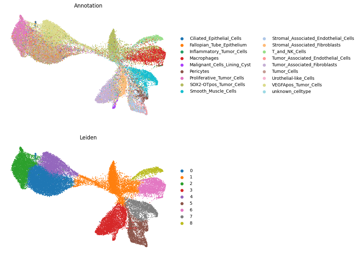
# Plot cell type annotations on UMAP
import matplotlib.pyplot as plt
import scanpy as sc

fig, axes = plt.subplots(2, 1, figsize=(7, 10))

sc.pl.umap(
    sdata.tables["table_transcriptomics_annotated"],
    color="annotation",
    legend_loc="right margin",
    frameon=False,
    size=12,
    ax=axes[0],
    show=False,
)
axes[0].set_title("Annotation")

sc.pl.umap(
    sdata.tables["table_transcriptomics_annotated"],
    color="leiden",
    legend_loc="right margin",
    frameon=False,
    size=12,
    ax=axes[1],
    show=False,
)
axes[1].set_title("Leiden")

Text(0.5, 1.0, 'Leiden')

# Plot annotation spatially

fig, ax = plt.subplots(1, 1, figsize=(10, 10))

hp.pl.plot_sdata(
    sdata,
    ax=ax,
    image_name="clahe",
    channel="DAPI",
    table_name="table_transcriptomics_annotated",
    labels_name="nucleus_segmentation_mask",
    color="annotation",
    # crd=(min_x, max_x, min_y, max_y),
    to_coordinate_system="global",
    render_images_kwargs={"cmap": "grey"},
    render_labels_kwargs={"fill_alpha": 1},
    show_kwargs={"title": "Annotation", "colorbar": False},
)

ax.axis("off")

(np.float64(10000.0),
 np.float64(20000.0),
 np.float64(28000.0),
 np.float64(18000.0))

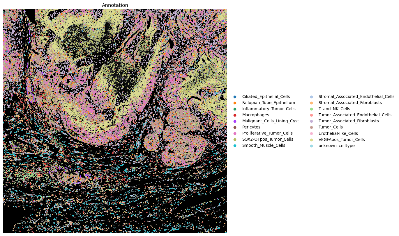
# Let's inspect the cell type counts and percentages
counts = (
    sdata.tables["table_transcriptomics_annotated"].obs["annotation"].value_counts()
)
percentages = (
    sdata.tables["table_transcriptomics_annotated"]
    .obs["annotation"]
    .value_counts(normalize=True)
    * 100
)

cluster_summary = pd.DataFrame({"count": counts, "percentage": percentages.round(2)})

print(cluster_summary)

                                      count  percentage
annotation                                             
SOX2-OTpos_Tumor_Cells                 6046       18.05
Tumor_Cells                            5352       15.97
VEGFApos_Tumor_Cells                   5005       14.94
Proliferative_Tumor_Cells              2873        8.58
Tumor_Associated_Fibroblasts           2574        7.68
Macrophages                            2076        6.20
Smooth_Muscle_Cells                    1969        5.88
Stromal_Associated_Fibroblasts         1634        4.88
Stromal_Associated_Endothelial_Cells   1496        4.47
Fallopian_Tube_Epithelium              1148        3.43
unknown_celltype                        749        2.24
T_and_NK_Cells                          628        1.87
Pericytes                               615        1.84
Tumor_Associated_Endothelial_Cells      407        1.21
Urothelial-like_Cells                   311        0.93
Malignant_Cells_Lining_Cyst             220        0.66
Inflammatory_Tumor_Cells                214        0.64
Ciliated_Epithelial_Cells               186        0.56

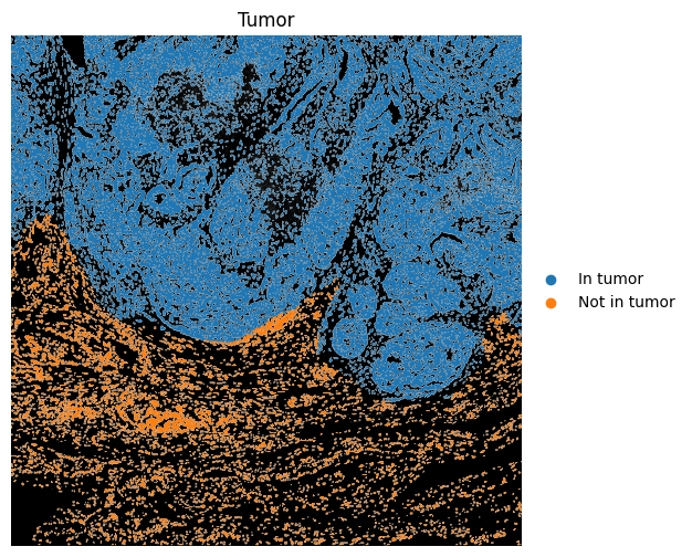
6.2 Using region annotations

We can use region annotations to assign which cells occurs within or outside those regions, calculate distances to the edge of the annotation, filter cells based on their relation the region annotation, etc.

Note that one should be very careful here to consider all coordinate spaces and transformations involved to make sure the results are correct.

import geopandas as gpd
from spatialdata.models import TableModel

# Get spatial coordinates
spatial_coords = sdata.tables["table_transcriptomics_annotated"].obsm["spatial"]
spatial_coords_df = pd.DataFrame(
    spatial_coords,
    columns=["x", "y"],
    index=sdata.tables["table_transcriptomics_annotated"].obs.index,
)

# Build points GeoDataFrame from centroids
points = gpd.GeoDataFrame(
    spatial_coords_df.copy(),
    geometry=gpd.points_from_xy(spatial_coords_df["x"], spatial_coords_df["y"]),
)

# If tumor has multiple polygons, combine once
tumor_union = sdata.shapes["tumor"].geometry.union_all()

# Vectorized test
in_tumor_mask = points.geometry.within(tumor_union)

yes_no = pd.Series(in_tumor_mask).map({True: "In tumor", False: "Not in tumor"})
cat_type = pd.CategoricalDtype(categories=["In tumor", "Not in tumor"], ordered=True)

sdata.tables["table_transcriptomics_annotated"].obs["in_tumor"] = yes_no.astype(
    cat_type
).values

region = sdata.tables["table_transcriptomics_annotated"].uns[TableModel.ATTRS_KEY][
    TableModel.REGION_KEY
]

sdata = hp.tb.add_table(
    sdata,
    adata=sdata.tables["table_transcriptomics_annotated"],
    output_table_name="table_transcriptomics_annotated",
    region=region,
    overwrite=True,
)

fig, ax = plt.subplots(1, 1, figsize=(6, 6))

ax = hp.pl.plot_sdata(
    sdata,
    image_name="clahe",
    channel="DAPI",
    table_name="table_transcriptomics_annotated",
    labels_name="nucleus_segmentation_mask",
    color="in_tumor",
    # crd=(min_x, max_x, min_y, max_y),
    to_coordinate_system="global",
    render_images_kwargs={"cmap": "grey", "colorbar": False},
    render_labels_kwargs={"fill_alpha": 1},
    show_kwargs={"title": "Tumor", "colorbar": True},
    ax=ax,
)

ax.axis("off")

(np.float64(10000.0),
 np.float64(20000.0),
 np.float64(28000.0),
 np.float64(18000.0))

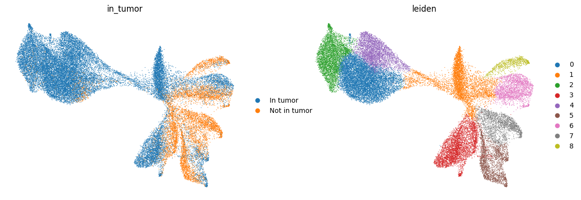
sc.pl.umap(
    sdata.tables["table_transcriptomics_annotated"],
    color=["in_tumor", "leiden"],
    show=True,
    frameon=False,
)

# copy of stringdtype in adata.uns can lead to kernel crash for numpy<2.2.5 (https://github.com/numpy/numpy/issues/28609)
del sdata.tables["table_transcriptomics_annotated"].uns["leiden_colors"]
del sdata.tables["table_transcriptomics_annotated"].uns["in_tumor_colors"]
del sdata.tables["table_transcriptomics_annotated"].uns["annotation_colors"]

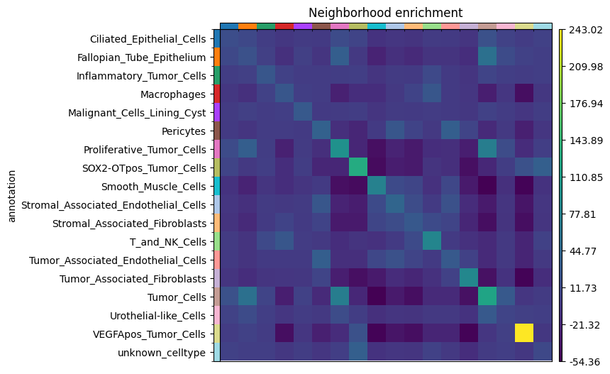
6.3 Neighborhood Niche Analysis and Squidpy Integration

Neighborhood enrichment in Squidpy tests whether annotated cell populations are found next to each other more or less often than expected by chance. The result depends on how we define the spatial neighborhood graph. Below, we first build a radius-based graph with r = 100. Here, the radius is interpreted in pixel coordinates because the cell centroids stored in the AnnData table are also in pixel space. We then reuse the same connectivity matrix in harpy.tb.nhood_kmeans and harpy.tb.nhood_lda to derive neighborhood-composition clusters and finally compute Squidpy’s neighborhood enrichment on that same graph.

import squidpy as sq

# First, we create a radius-based spatial graph.
r = 100
sq.gr.spatial_neighbors(
    adata=sdata.tables["table_transcriptomics_annotated"],
    spatial_key="spatial",  # .obsm["spatial"] stores cell centroids in pixel coordinates.
    coord_type="generic",
    radius=r,
    key_added=f"radius_{r}",
)

INFO     Creating graph using `generic` coordinates and `None` transform and `1` libraries.

import harpy as hp

sdata = hp.tb.nhood_kmeans(
    sdata,
    table_name="table_transcriptomics_annotated",
    output_table_name="table_transcriptomics_annotated",
    cluster_key="annotation",
    connectivity_key=f"radius_{r}",
    composition_key="nhood_composition",
    key_added="nhood_kmeans",
    n_clusters=6,
    nan_label="Isolated",  # Label assigned to isolated cells with zero graph degree.
    overwrite=True,
)

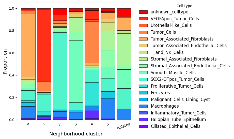
# Plot the cell-type composition of each neighborhood cluster.
pivot_df = sdata.tables["table_transcriptomics_annotated"].obs.pivot_table(
    index="nhood_kmeans", columns="annotation", aggfunc="size", fill_value=0
)
proportions = pivot_df.div(pivot_df.sum(axis=1), axis=0)
proportions = proportions.reset_index()

ax = proportions.plot.bar(
    x="nhood_kmeans",
    stacked=True,
    cmap="rainbow",
    figsize=(6, 6),
    width=0.9,
    edgecolor="black",
    linewidth=0.5,
)

fig = ax.get_figure()

ax.set_xlabel("Neighborhood cluster", fontsize=14, color="black")
ax.set_ylabel("Proportion", fontsize=14, color="black")
ax.tick_params(axis="x", rotation=20, colors="black")
ax.tick_params(axis="y", colors="black")

handles, labels = ax.get_legend_handles_labels()
ax.legend(
    handles[::-1],
    labels[::-1],
    title="Cell type",
    bbox_to_anchor=(1, 1.02),
    fontsize=12,
    labelcolor="black",
    frameon=False,
)

<matplotlib.legend.Legend at 0x145bcea50>

fig, ax = plt.subplots(1, 1, figsize=(10, 10))

ax = hp.pl.plot_sdata(
    sdata,
    image_name="clahe",
    channel="DAPI",
    table_name="table_transcriptomics_annotated",
    labels_name="nucleus_segmentation_mask",
    color="nhood_kmeans",
    # crd=(min_x, max_x, min_y, max_y),
    to_coordinate_system="global",
    render_images_kwargs={"cmap": "grey", "colorbar": False},
    render_labels_kwargs={"fill_alpha": 1},
    show_kwargs={"title": "Neighborhood clusters (Kmeans)", "colorbar": True},
    ax=ax,
)

ax.axis("off")

(np.float64(10000.0),
 np.float64(20000.0),
 np.float64(28000.0),
 np.float64(18000.0))

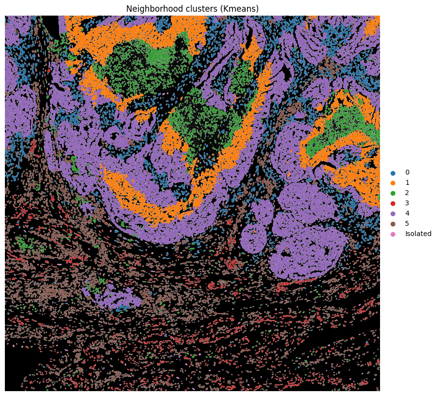
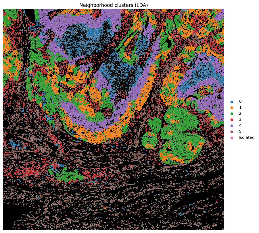
Harpy also implements neighborhood clustering into niche topics using LDA.

import harpy as hp

sdata = hp.tb.nhood_lda(
    sdata,
    table_name="table_transcriptomics_annotated",
    output_table_name="table_transcriptomics_annotated",
    cluster_key="annotation",
    connectivity_key=f"radius_{r}",
    counts_key="nhood_counts",
    key_added="nhood_lda",
    n_topics=6,
    nan_label="Isolated",  # Label assigned to isolated cells with zero graph degree.
    overwrite=True,
)

fig, ax = plt.subplots(1, 1, figsize=(10, 10))

ax = hp.pl.plot_sdata(
    sdata,
    image_name="clahe",
    channel="DAPI",
    table_name="table_transcriptomics_annotated",
    labels_name="nucleus_segmentation_mask",
    color="nhood_lda",
    # crd=(min_x, max_x, min_y, max_y),
    to_coordinate_system="global",
    render_images_kwargs={"cmap": "grey", "colorbar": False},
    render_labels_kwargs={"fill_alpha": 1},
    show_kwargs={"title": "Neighborhood clusters (LDA)", "colorbar": True},
    ax=ax,
)

ax.axis("off")

(np.float64(10000.0),
 np.float64(20000.0),
 np.float64(28000.0),
 np.float64(18000.0))

# Calculate nhood enrichment on the same radius-based graph.
adata = sdata.tables["table_transcriptomics_annotated"]
sq.gr.nhood_enrichment(
    adata,
    cluster_key="annotation",
    connectivity_key=f"radius_{r}",
)

# Plot neighborhood enrichment.
sq.pl.nhood_enrichment(
    adata,
    cluster_key="annotation",
    figsize=(5, 5),
    mode="zscore",
)