Example spatial transcriptomics (Xenium)

Data downloaded from 10x Genomics (accessed 25/11/2025): https://www.10xgenomics.com/datasets/xenium-prime-ffpe-human-ovarian-cancer

1. Read in the data

import os

import harpy as hp

path_sdata = os.path.join(
    os.environ.get("TMPDIR"), "sdata.zarr"
)  # or pick a path where the SpatialData object will be backed.

# takes around 7 minutes
sdata = hp.datasets.xenium_human_ovarian_cancer(output=path_sdata)

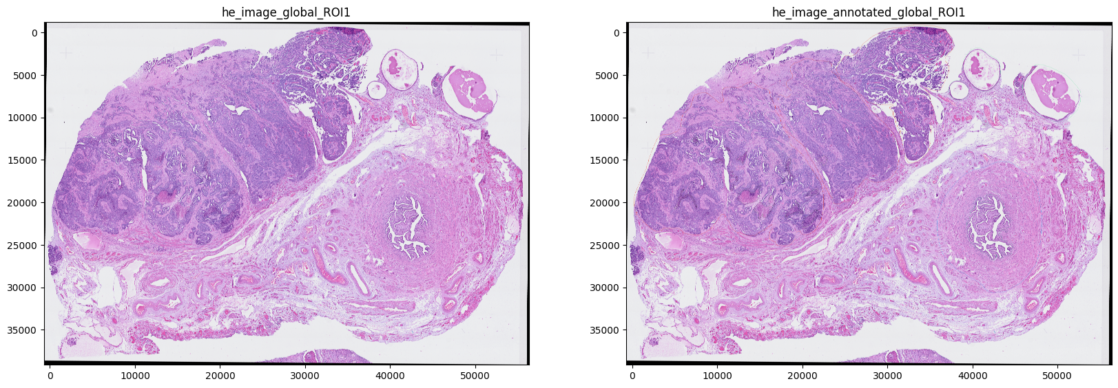
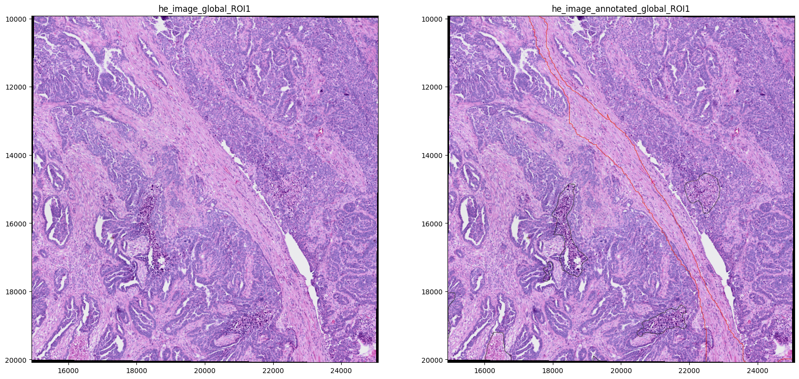
2. Plot the images

H&E and annotated H&E

import matplotlib.pyplot as plt

fig, axes = plt.subplots(1, 2, figsize=(20, 10))

image_name = ["he_image_global_ROI1", "he_image_annotated_global_ROI1"]

for _image_name, _ax in zip(image_name, axes, strict=True):
    show_kwargs = {
        "title": _image_name,
        "colorbar": False,
    }
    ax = hp.pl.plot_sdata(
        sdata,
        image_name=_image_name,
        channel=["r", "g", "b"],
        to_coordinate_system="global_ROI1",  # or if you want to plot in micron coordinates, specify "global_ROI1_micron"
        show_kwargs=show_kwargs,
        ax=_ax,
    )

INFO     Rasterizing image for faster rendering.                                                                   
INFO     Rasterizing image for faster rendering.

import matplotlib.pyplot as plt

fig, axes = plt.subplots(1, 2, figsize=(20, 10))

show_kwargs = {"colorbar": False}

image_name = ["he_image_global_ROI1", "he_image_annotated_global_ROI1"]
for _image_name, _ax in zip(image_name, axes, strict=True):
    show_kwargs = {
        "title": _image_name,
        "colorbar": False,
    }
    ax = hp.pl.plot_sdata(
        sdata,
        image_name=_image_name,
        crd=[15000, 25000, 10000, 20000],
        channel=["r", "g", "b"],
        to_coordinate_system="global_ROI1",
        show_kwargs=show_kwargs,
        ax=_ax,
    )

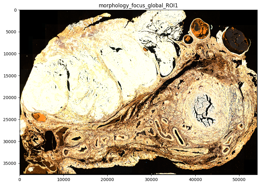
Morphology focus

This is the image that is used for segmentation.

import matplotlib.pyplot as plt

fig, ax = plt.subplots(1, 1, figsize=(10, 10))

image_name = "morphology_focus_global_ROI1"
channel = hp.im.get_dataarray(sdata, element_name=image_name).c.data.tolist()

show_kwargs = {
    "title": image_name,
    "colorbar": False,
}
ax = hp.pl.plot_sdata(
    sdata,
    image_name=image_name,
    channel=channel,
    to_coordinate_system="global_ROI1",  # or if you want to plot in micron coordinates, specify "global_ROI1_micron"
    show_kwargs=show_kwargs,
    ax=ax,
)

INFO     Rasterizing image for faster rendering.                                                                   
INFO     Your image has 4 channels. Sampling categorical colors and using multichannel strategy 'stack' to render.

2. Visualize the transcripts

import matplotlib.pyplot as plt

fig, ax = plt.subplots(1, 1, figsize=(8, 8))

render_images_kwargs = {
    "cmap": "binary",
}
show_kwargs = {
    "title": "transcripts",
    "colorbar": False,
}

hp.pl.plot_sdata_genes(
    sdata,
    points_name="transcripts_global_ROI1",
    image_name="morphology_focus_global_ROI1",
    channel="DAPI",
    genes=None,  # plot all genes
    color="cornflowerblue",
    size=0.1,
    frac=0.01,  # only plot 1% of them
    to_coordinate_system="global_ROI1",
    show_kwargs=show_kwargs,
    render_images_kwargs=render_images_kwargs,
    ax=ax,
)

INFO     Value for parameter 'color' appears to be a color, using it as such.                                      
INFO     Rasterizing image for faster rendering.
INFO     Using 'datashader' backend with 'None' as reduction method to speed up plotting. Depending on the         
         reduction method, the value range of the plot might change. Set method to 'matplotlib' do disable this    
         behaviour.

<Axes: title={'center': 'transcripts'}>

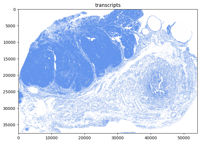
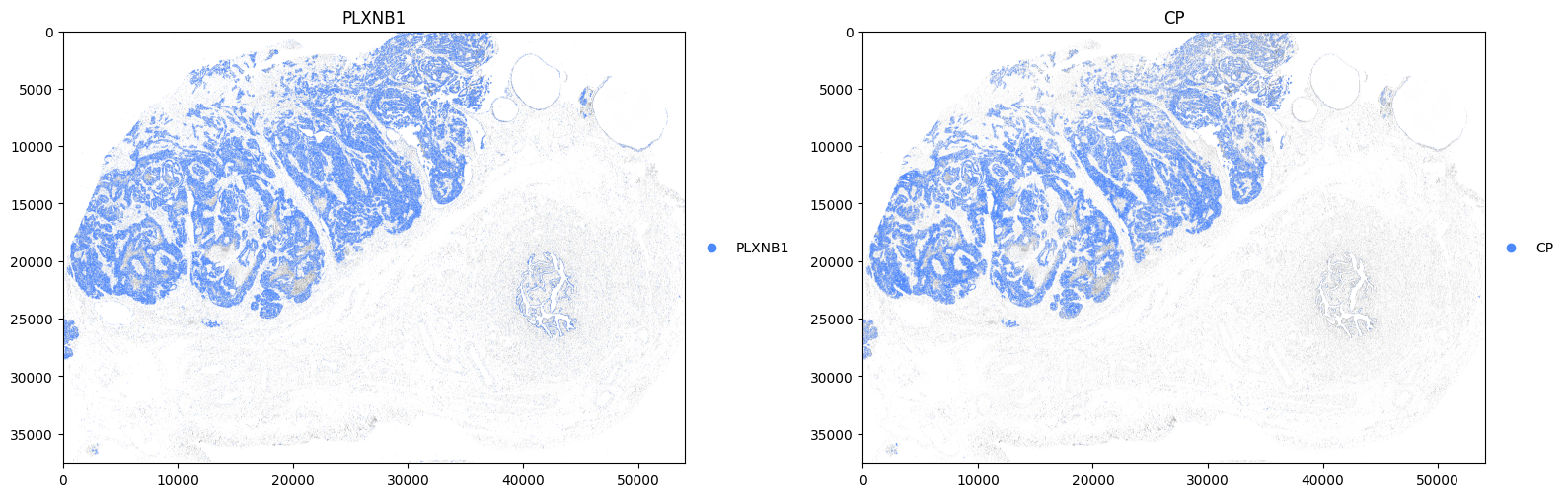
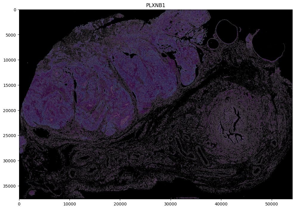
Now plot some genes associated with tumor cells.

import matplotlib.pyplot as plt

fig, axes = plt.subplots(1, 2, figsize=(16, 8))

render_images_kwargs = {
    "cmap": "binary",
}

for gene, ax in zip(["PLXNB1", "CP"], axes, strict=True):
    show_kwargs = {
        "title": gene,
        "colorbar": False,
    }

    hp.pl.plot_sdata_genes(
        sdata,
        points_name="transcripts_global_ROI1",
        image_name="morphology_focus_global_ROI1",
        channel="DAPI",
        genes=[
            gene
        ],  #  You could specify a list of genes here. But note that if they occur at same location, they will plotted onto each other.
        palette=["#4D88FF"],
        size=0.1,
        frac=None,
        to_coordinate_system="global_ROI1",
        show_kwargs=show_kwargs,
        render_images_kwargs=render_images_kwargs,
        ax=ax,
    )
plt.tight_layout()
plt.show()

INFO     Rasterizing image for faster rendering.
INFO     input has more than 103 categories. Uniform 'grey' color will be used for all categories.                 
INFO     Using 'datashader' backend with 'None' as reduction method to speed up plotting. Depending on the         
         reduction method, the value range of the plot might change. Set method to 'matplotlib' do disable this    
         behaviour.
INFO     Rasterizing image for faster rendering.                                                                   
INFO     input has more than 103 categories. Uniform 'grey' color will be used for all categories.                 
INFO     Using 'datashader' backend with 'None' as reduction method to speed up plotting. Depending on the         
         reduction method, the value range of the plot might change. Set method to 'matplotlib' do disable this    
         behaviour.

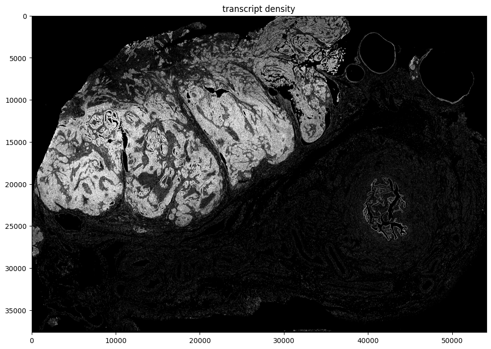
Calculate the transcript density

sdata = hp.im.transcript_density(
    sdata,
    points_name="transcripts_global_ROI1",
    image_name="morphology_focus_global_ROI1",
    output_image_name="transcript_density",
    to_coordinate_system="global_ROI1",
    scale_factors=[2, 2, 2, 2],
    overwrite=True,
)

import numpy as np

import dask.array as da

from matplotlib.colors import Normalize

scale = None  # auto pick scale by spatialdata-plot
image_name = "transcript_density"

fig, ax = plt.subplots(1, 1, figsize=(10, 10))

channel = 0
se = hp.im.get_dataarray(sdata, element_name=image_name)
_channel_idx = np.where(se.c.data == channel)[0].item()
vmax = da.percentile(se.data[_channel_idx].flatten(), q=95).compute()
norm = Normalize(vmax=vmax, clip=False)
print(norm)

crd = None
sdata_to_plot = sdata.subset(element_names=[image_name])

render_images_kwargs = {"cmap": "grey", "scale": scale, "norm": norm}
show_kwargs = {
    "title": "transcript density",
    "colorbar": False,
}
ax = hp.pl.plot_sdata(
    sdata_to_plot,
    image_name=image_name,
    channel=channel,
    crd=crd,
    to_coordinate_system="global_ROI1",
    render_images_kwargs=render_images_kwargs,
    show_kwargs=show_kwargs,
    ax=ax,
)

plt.tight_layout()
plt.show()

<matplotlib.colors.Normalize object at 0x7f4e992eae40>
INFO     Rasterizing image for faster rendering.

3. Segmentation

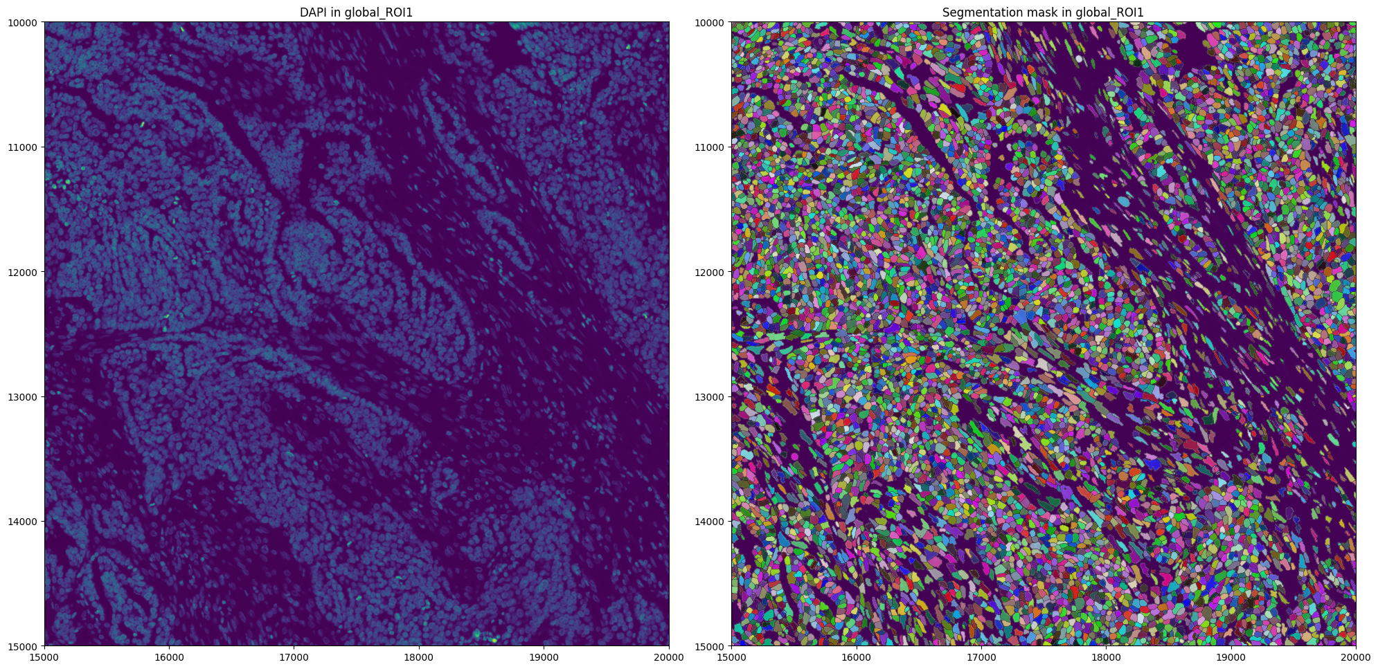
Segmentation is already provided by 10x Genomics. We will inspect these segmentation masks, and also illustate how the user could generate segmentation masks using harpy.

First visualize segmentation masks provided by 10x Genomics.

fig, axes = plt.subplots(1, 2, figsize=(20, 10))

channel = "DAPI"
image_name = "morphology_focus_global_ROI1"
labels_name = "cell_labels_global_ROI1"

crd = [15000, 20000, 10000, 15000]

to_coordinate_system = "global_ROI1"

render_images_kwargs = {"cmap": "viridis"}
render_labels_kwargs = {"fill_alpha": 0.6, "outline_alpha": 0.4}
show_kwargs = {"title": f"DAPI in {to_coordinate_system}", "colorbar": False}

hp.pl.plot_sdata(
    sdata,
    image_name=image_name,
    crd=crd,
    to_coordinate_system=to_coordinate_system,
    channel=channel,
    render_images_kwargs=render_images_kwargs,
    show_kwargs=show_kwargs,
    ax=axes[0],
)
# _ax.axis("off")

show_kwargs = {
    "title": f"Segmentation mask in {to_coordinate_system}",
    "colorbar": False,
}
hp.pl.plot_sdata(
    sdata,
    image_name=image_name,
    labels_name=labels_name,
    crd=crd,
    to_coordinate_system=to_coordinate_system,
    channel=channel,
    render_images_kwargs=render_images_kwargs,
    render_labels_kwargs=render_labels_kwargs,
    show_kwargs=show_kwargs,
    ax=axes[1],
)
# _ax.axis("off")

plt.tight_layout()
plt.show()

In many cases, you want to generate these segmentation masks yourself. Therefore, for illustration purposes, we show how to segment using Cellpose via harpy.im.segment, and how to generate an AnnData table using hp.tb.allocate.

Make sure to install Cellpose before running the following cell (pip install cellpose).

import os
import torch
from dask.distributed import Client, LocalCluster

if torch.cuda.is_available():
    from dask_cuda import LocalCUDACluster  # pip install dask-cuda

    # One worker per GPU; each worker will be pinned to a single GPU.
    cluster = LocalCUDACluster(
        CUDA_VISIBLE_DEVICES=[0],  # or [0,1],...etc
        n_workers=1,  # 2 if [0,1],...etc
        threads_per_worker=1,
        memory_limit="32GB",
        local_directory=os.environ.get("TMPDIR"),
    )
else:
    # cpu/mps fall back
    from dask.distributed import LocalCluster

    cluster = LocalCluster(
        n_workers=1
        if torch.backends.mps.is_available()
        else 8,  # If mps/cuda device available, it is better to increase chunk size to maximal value that fits on the gpu, and set n_workers to 1.
        # For this dummy example, we only have one chunk, so setting n_workers>1, has no effect.
        threads_per_worker=1,
        memory_limit="32GB",
        local_directory=os.environ.get("TMPDIR"),
    )

client = Client(cluster)

print(client.dashboard_link)

sdata = hp.im.segment(
    sdata,
    image_name="morphology_focus_global_ROI1",  # note, currently cellpose only supports segmentation of 3 channels. So the channel at index -1 will not be used (AlphaSMA/Vimentin)
    depth=200,
    model=hp.im.cellpose_callable,
    # parameters that will be passed to the callable cellpose_callable
    diameter=50,
    flow_threshold=0.9,
    cellprob_threshold=-4,
    output_labels_name="cell_labels_harpy_global_ROI1",
    output_shapes_name=None,
    crd=[15000, 20000, 10000, 15000],
    # region to segment [x_min, xmax, y_min, y_max], must be defined in pixel coordinates, e.g. specify the pixel coordinate system
    to_coordinate_system="global_ROI1",
    overwrite=True,
)
client.close()

http://127.0.0.1:8787/status

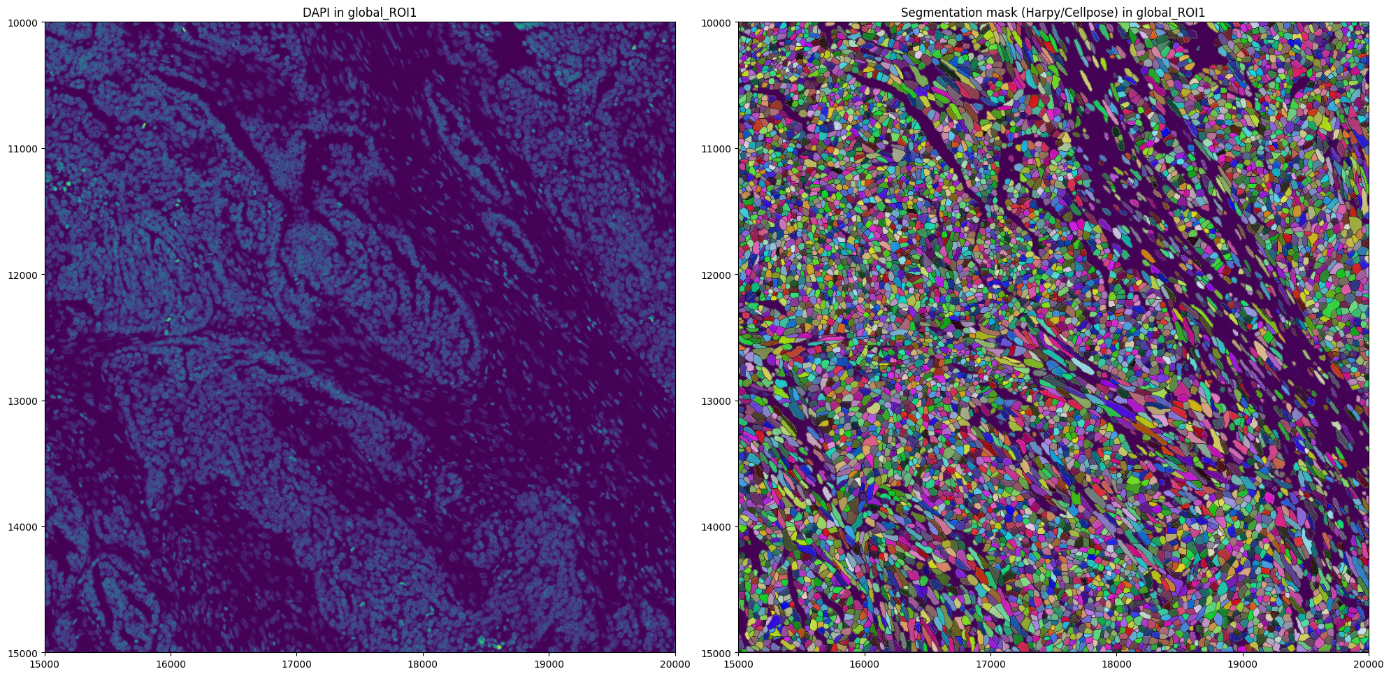
Lets inspect the segmentation masks we generated.

import matplotlib.pyplot as plt

fig, axes = plt.subplots(1, 2, figsize=(20, 10))

channel = "DAPI"
image_name = "morphology_focus_global_ROI1"
labels_name = "cell_labels_harpy_global_ROI1"

crd = [15000, 20000, 10000, 15000]

to_coordinate_system = "global_ROI1"

render_images_kwargs = {"cmap": "viridis"}
render_labels_kwargs = {"fill_alpha": 0.6, "outline_alpha": 0.4}
show_kwargs = {"title": f"DAPI in {to_coordinate_system}", "colorbar": False}

hp.pl.plot_sdata(
    sdata,
    image_name=image_name,
    crd=crd,
    to_coordinate_system=to_coordinate_system,
    channel=channel,
    render_images_kwargs=render_images_kwargs,
    show_kwargs=show_kwargs,
    ax=axes[0],
)
# _ax.axis("off")

show_kwargs = {
    "title": f"Segmentation mask (Harpy/Cellpose) in {to_coordinate_system}",
    "colorbar": False,
}
hp.pl.plot_sdata(
    sdata,
    image_name=image_name,
    labels_name=labels_name,
    crd=crd,
    to_coordinate_system=to_coordinate_system,
    channel=channel,
    render_images_kwargs=render_images_kwargs,
    render_labels_kwargs=render_labels_kwargs,
    show_kwargs=show_kwargs,
    ax=axes[1],
)
# _ax.axis("off")

plt.tight_layout()
plt.show()

INFO     Rasterizing image for faster rendering.

4. Create the AnnData table

Below we illustrate how an AnnData table can be created using this custom generated segmentation mask via the harpy function harpy.tb.allocate.

from dask.distributed import Client, LocalCluster

cluster = LocalCluster(
    n_workers=16,
    threads_per_worker=1,
    processes=True,
    memory_limit="8GB",
    local_directory=os.environ.get("TMPDIR"),  # folder where dask will spill to disk
)

client = Client(cluster)

sdata = sdata = hp.tb.allocate(
    sdata,
    labels_name="cell_labels_harpy_global_ROI1",
    points_name="transcripts_global_ROI1",
    output_table_name="table_harpy_global_ROI1",
    to_coordinate_system="global_ROI1",  # Do allocation step in the intrinsic pixel coordinate system,
    append=False,
    overwrite=True,
    update_shapes_elements=False,
)

client.close()

5. Preprocess the AnnData table

We proceed working with the AnnData table provided by 10x Genomics. But the same logic applies to a custom generated AnnData table.

labels_name = "cell_labels_global_ROI1"
table_name = "table_global_ROI1"
points_name = "transcripts_global_ROI1"

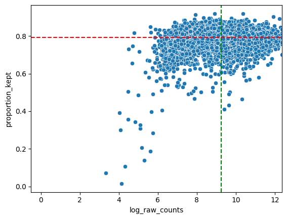
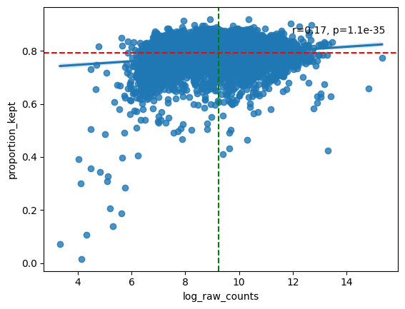
filtered = hp.qc.analyse_genes_left_out(
    sdata,
    labels_name=labels_name,
    table_name=table_name,
    points_name=points_name,
    to_coordinate_system=to_coordinate_system,
)

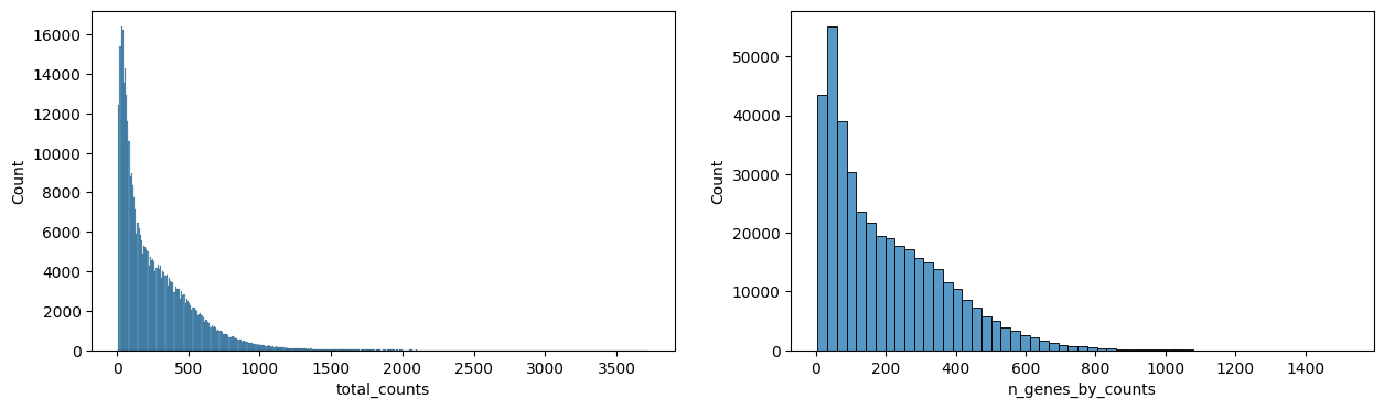
We proceed with filtering of cells with low transcript count, and genes with low cell count; normalization using cell size; a log transformation; and scaling such that the data has mean zero and a variance of one.

sdata = hp.tb.preprocess_transcriptomics(
    sdata,
    labels_name=labels_name,
    table_name=table_name,
    output_table_name="table_global_ROI1_preprocessed",
    size_norm=True,
    update_shapes_elements=False,
    overwrite=True,
)

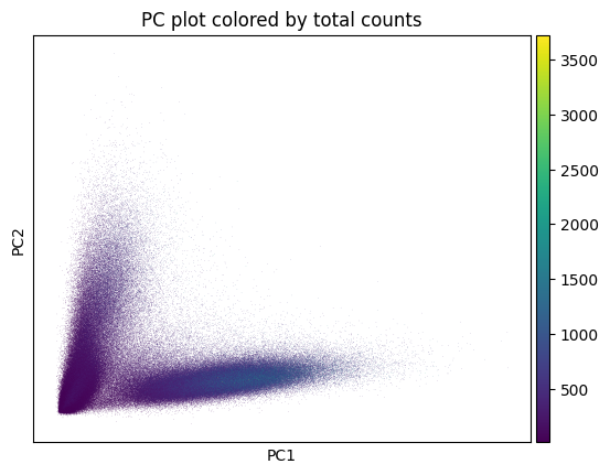
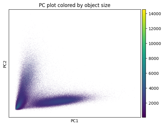
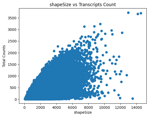
hp.pl.preprocess_transcriptomics(
    sdata,
    table_name="table_global_ROI1_preprocessed",
)

Visualize the expression after preprocessing.

# show expression after preprocessing;
import matplotlib.pyplot as plt

channel = "DAPI"
image_name = "morphology_focus_global_ROI1"
labels_name = "cell_labels_global_ROI1"
table_name = "table_global_ROI1_preprocessed"

fig, axes = plt.subplots(1, 1, figsize=(10, 10))

to_coordinate_system = to_coordinate_system
scale = None  # auto pick scale by spatialdata-plot
color = "PLXNB1"  # visualize expression of specific genes
crd = None

# if points in, query is slow, so remove them for plotting
sdata_to_plot = sdata.subset(element_names=[image_name, labels_name, table_name])

render_images_kwargs = {"cmap": "grey", "norm": None, "scale": scale}
render_labels_kwargs = {"fill_alpha": 0.5, "outline_alpha": 0.4, "scale": scale}
show_kwargs = {
    "title": color,
    "colorbar": False,
}
axes = hp.pl.plot_sdata(
    sdata_to_plot,
    image_name=image_name,
    labels_name=labels_name,
    table_name=table_name,
    color=color,
    channel=channel,
    crd=crd,
    render_images_kwargs=render_images_kwargs,
    show_kwargs=show_kwargs,
    ax=axes,
    to_coordinate_system=to_coordinate_system,
)

plt.tight_layout()
plt.show()

INFO     Rasterizing image for faster rendering.                                                                   
INFO     Rasterizing image for faster rendering.

6. Leiden clustering.

# takes around 40 minutes
# This can consume quite some RAM, as the AnnData table is in memory.

labels_name = "cell_labels_global_ROI1"
table_name = "table_global_ROI1_preprocessed"

sdata = hp.tb.leiden(
    sdata,
    labels_name=labels_name,
    table_name=table_name,
    output_table_name=table_name,
    overwrite=True,
)

sdata.tables["table_global_ROI1_preprocessed"].obs.head()

	transcript_counts	control_probe_counts	genomic_control_counts	control_codeword_counts	unassigned_codeword_counts	deprecated_codeword_counts	total_counts	cell_area	nucleus_area	nucleus_count	...	cell_ID	group	n_genes_by_counts	log1p_n_genes_by_counts	log1p_total_counts	pct_counts_in_top_2_genes	pct_counts_in_top_5_genes	n_counts	shapeSize	leiden
cell_id
aaaaebmm-1	303	0	0	0	0	31	303.0	44.659533	31.835157	1.0	...	1	Proliferative Tumor Cells	246	5.509388	5.717028	7.260726	10.231023	303.0	989	3
aaaafhpp-1	311	0	0	0	0	28	311.0	57.664533	38.247345	1.0	...	2	Tumor Cells	255	5.545177	5.743003	2.893891	6.109325	311.0	1277	10
aaaahcem-1	301	0	0	0	0	32	301.0	39.827814	27.590470	1.0	...	3	Proliferative Tumor Cells	249	5.521461	5.710427	4.983389	8.637874	301.0	882	3
aaaakeoi-1	369	0	0	0	0	58	369.0	60.870627	38.879533	1.0	...	4	Proliferative Tumor Cells	306	5.726848	5.913503	3.252033	5.962060	369.0	1348	3
aaaalald-1	295	0	0	0	0	47	295.0	50.484689	46.510939	1.0	...	5	Tumor Cells	254	5.541264	5.690360	5.423729	8.813559	295.0	1118	10

5 rows × 23 columns

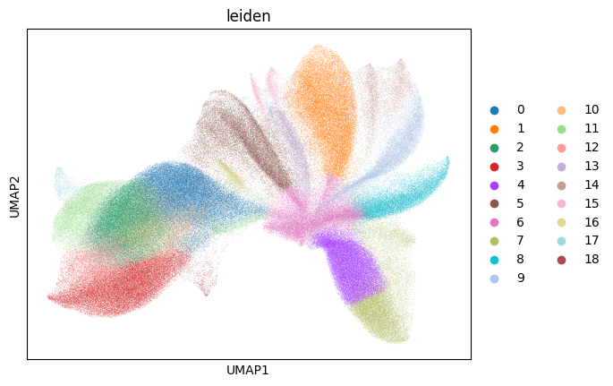
import scanpy as sc

sc.pl.umap(sdata.tables["table_global_ROI1_preprocessed"], color=["leiden"], show=True)
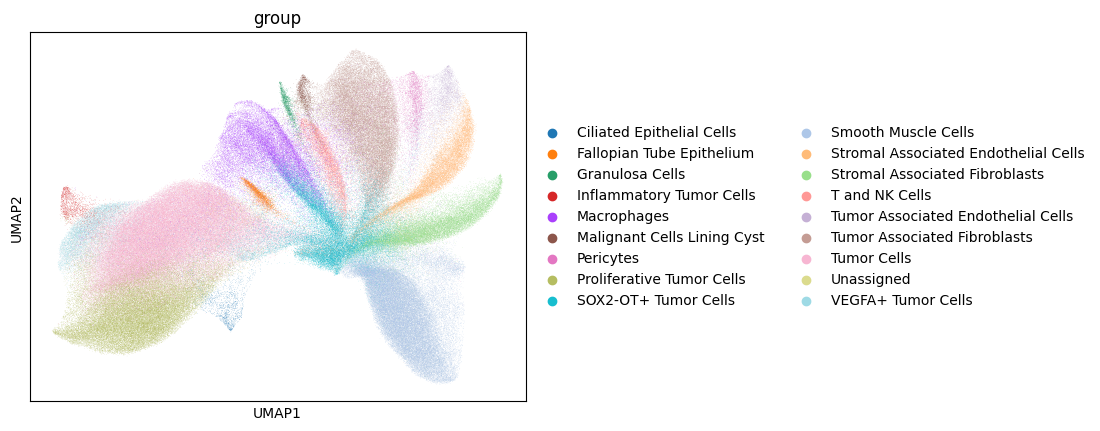
# this dataset is annotated, lets see how clusters correspond to cell type
sc.pl.umap(sdata.tables["table_global_ROI1_preprocessed"], color=["group"], show=True)

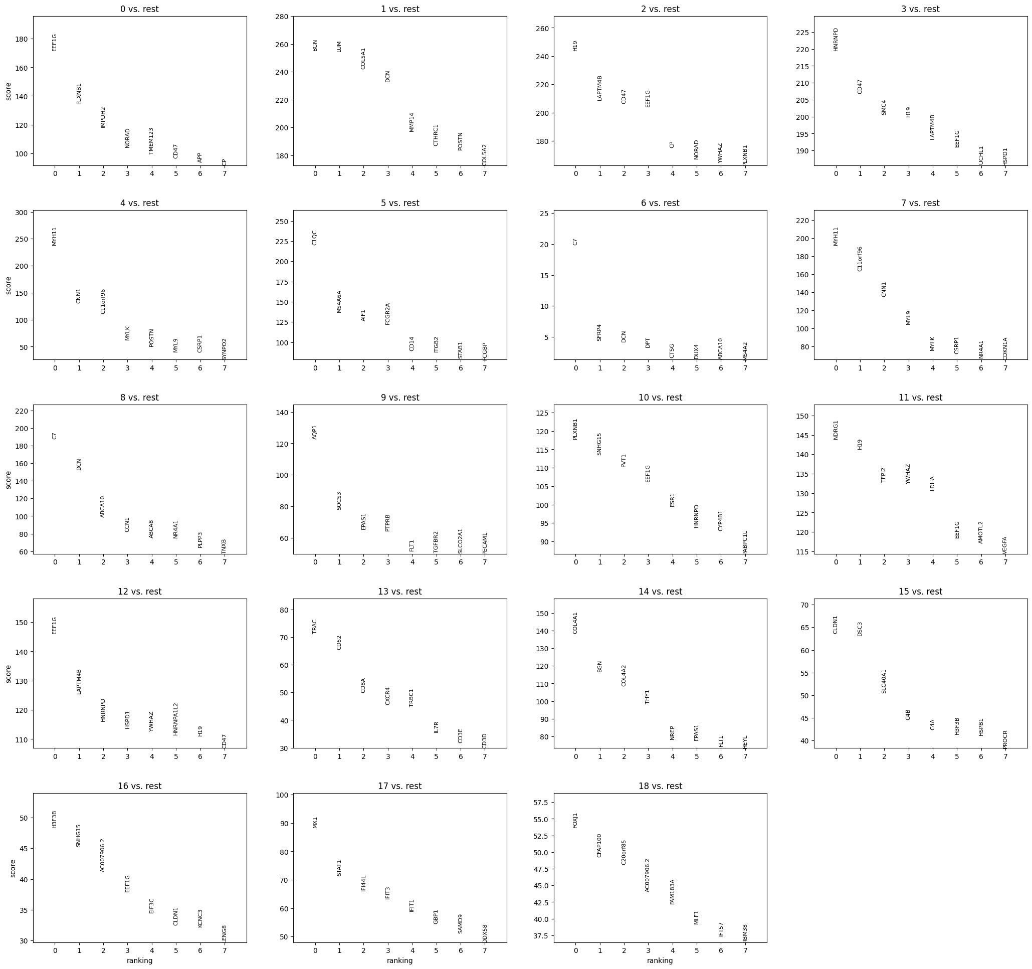
sc.pl.rank_genes_groups(
    sdata.tables["table_global_ROI1_preprocessed"], n_genes=8, sharey=False, show=False
)

[<Axes: title={'center': '0 vs. rest'}, ylabel='score'>,
 <Axes: title={'center': '1 vs. rest'}>,
 <Axes: title={'center': '2 vs. rest'}>,
 <Axes: title={'center': '3 vs. rest'}>,
 <Axes: title={'center': '4 vs. rest'}, ylabel='score'>,
 <Axes: title={'center': '5 vs. rest'}>,
 <Axes: title={'center': '6 vs. rest'}>,
 <Axes: title={'center': '7 vs. rest'}>,
 <Axes: title={'center': '8 vs. rest'}, ylabel='score'>,
 <Axes: title={'center': '9 vs. rest'}>,
 <Axes: title={'center': '10 vs. rest'}>,
 <Axes: title={'center': '11 vs. rest'}>,
 <Axes: title={'center': '12 vs. rest'}, ylabel='score'>,
 <Axes: title={'center': '13 vs. rest'}>,
 <Axes: title={'center': '14 vs. rest'}>,
 <Axes: title={'center': '15 vs. rest'}>,
 <Axes: title={'center': '16 vs. rest'}, xlabel='ranking', ylabel='score'>,
 <Axes: title={'center': '17 vs. rest'}, xlabel='ranking'>,
 <Axes: title={'center': '18 vs. rest'}, xlabel='ranking'>]

import matplotlib.pyplot as plt

channel = "DAPI"
image_name = "morphology_focus_global_ROI1"
labels_name = "cell_labels_global_ROI1"
table_name = "table_global_ROI1_preprocessed"
to_coordinate_system = "global_ROI1"


to_coordinate_system = to_coordinate_system
scale = None  # auto pick scale by spatialdata-plot
crd = None

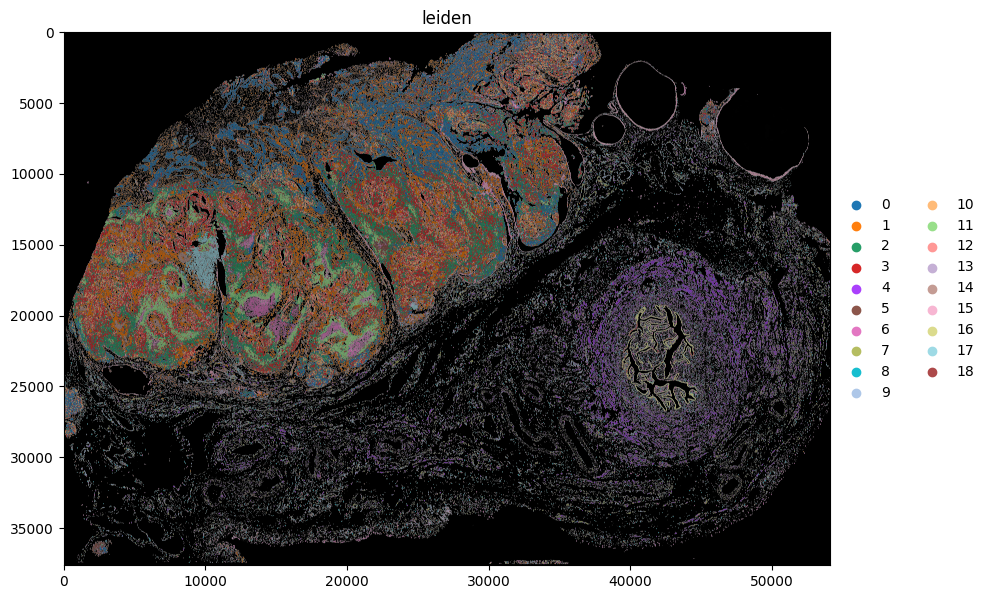
color = "leiden"

fig, ax = plt.subplots(1, 1, figsize=(10, 10))

# if points in, query is slow, so remove them for plotting
sdata_to_plot = sdata.subset(element_names=[image_name, labels_name, table_name])

render_images_kwargs = {"cmap": "grey", "norm": None, "scale": scale}
render_labels_kwargs = {"fill_alpha": 0.5, "outline_alpha": 0.4, "scale": scale}
show_kwargs = {
    "title": color,
    "colorbar": False,
}
ax = hp.pl.plot_sdata(
    sdata_to_plot,
    image_name=image_name,
    labels_name=labels_name,
    table_name=table_name,
    color=color,
    channel=channel,
    crd=crd,
    render_images_kwargs=render_images_kwargs,
    show_kwargs=show_kwargs,
    ax=ax,
    to_coordinate_system=to_coordinate_system,
)
# _ax.axis("off")

plt.tight_layout()
plt.show()

INFO     Rasterizing image for faster rendering.                                                                   
INFO     Rasterizing image for faster rendering.

import matplotlib.pyplot as plt

channel = "DAPI"
image_name = "morphology_focus_global_ROI1"
labels_name = "cell_labels_global_ROI1"
table_name = "table_global_ROI1_preprocessed"
to_coordinate_system = "global_ROI1"


to_coordinate_system = to_coordinate_system
scale = None  # auto pick scale by spatialdata-plot
crd = None

color = "group"

fig, ax = plt.subplots(1, 1, figsize=(20, 20))

# if points in, query is slow, so remove them for plotting
sdata_to_plot = sdata.subset(element_names=[image_name, labels_name, table_name])

render_images_kwargs = {"cmap": "grey", "norm": None, "scale": scale}
render_labels_kwargs = {"fill_alpha": 0.5, "outline_alpha": 0.4, "scale": scale}
show_kwargs = {
    "title": color,
    "colorbar": False,
}
ax = hp.pl.plot_sdata(
    sdata_to_plot,
    image_name=image_name,
    labels_name=labels_name,
    table_name=table_name,
    color=color,
    channel=channel,
    crd=crd,
    render_images_kwargs=render_images_kwargs,
    show_kwargs=show_kwargs,
    ax=ax,
    to_coordinate_system=to_coordinate_system,
)
# _ax.axis("off")

plt.tight_layout()
plt.show()

INFO     Rasterizing image for faster rendering.                                                                   
INFO     Rasterizing image for faster rendering.

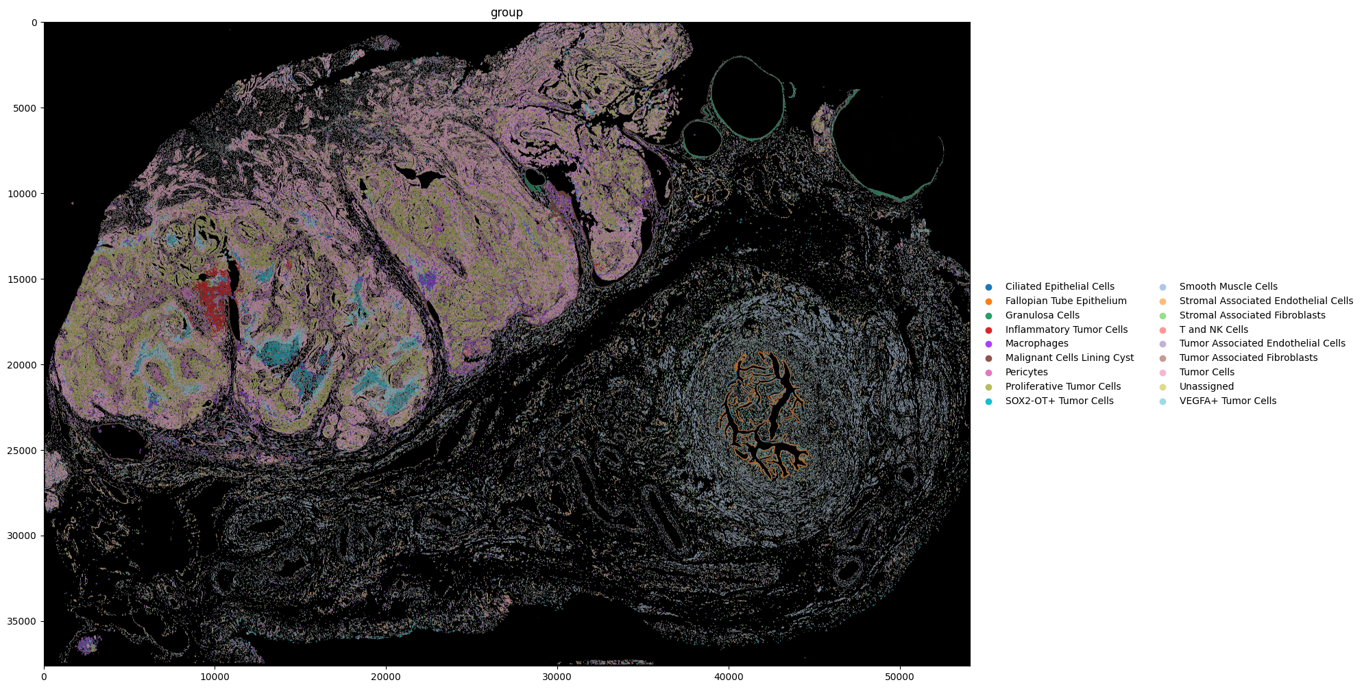
Note the correspondence between Leiden cluster 17, and the Inflammatory Tumor Cells.

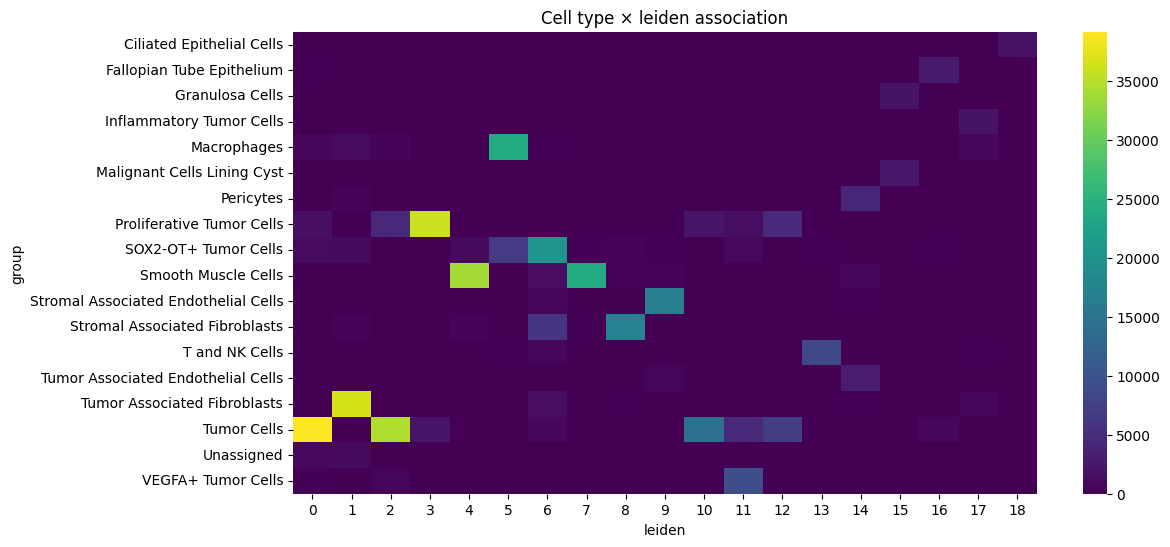
We also estimate the correlation between leiden clusters and the annotated cell type.

import matplotlib.pyplot as plt
import numpy as np
import pandas as pd
import seaborn as sns
from scipy.stats import chi2_contingency

table_name = "table_global_ROI1_preprocessed"
cluster_key = "leiden"
cell_type_key = "group"

df = sdata[table_name].obs

df = df[~df[cell_type_key].isna()]

contingency = pd.crosstab(df[cell_type_key], df[cluster_key])

# chi squared test
chi2, p, dof, expected = chi2_contingency(contingency)


# cramers v
def _cramers_v(confusion_matrix):
    chi2 = chi2_contingency(confusion_matrix)[0]
    n = confusion_matrix.sum().sum()
    phi2 = chi2 / n
    r, k = confusion_matrix.shape
    return np.sqrt(phi2 / min(k - 1, r - 1))


print("Cramers v:", _cramers_v(contingency))

print("Chi-squared statistic:", chi2)
print("p-value:", p)

plt.figure(figsize=(12, 6))
sns.heatmap(contingency, cmap="viridis")
plt.title(f"Cell type × {cluster_key} association")
plt.show()

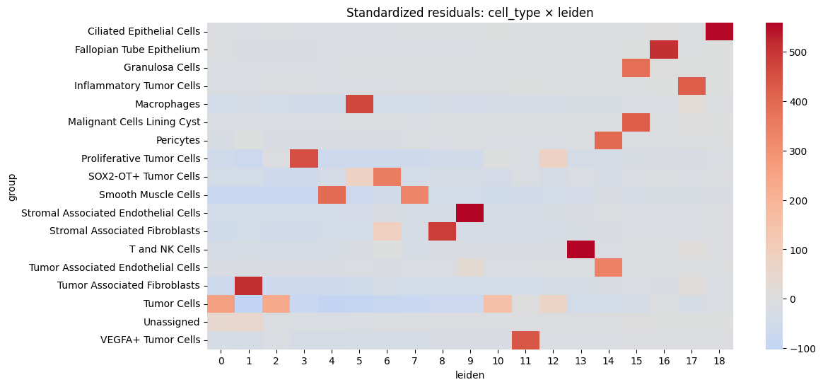
# Calculate standardized residuals
residuals = (contingency - expected) / np.sqrt(expected)

residuals_df = pd.DataFrame(
    residuals, index=contingency.index, columns=contingency.columns
)

resid_long = residuals_df.stack().reset_index()
resid_long.columns = ["cell_type", cluster_key, "std_residual"]

# Sort by strength of deviation
resid_long["abs_resid"] = resid_long["std_residual"].abs()
top_effects = resid_long.sort_values("abs_resid", ascending=False).head(20)
print(top_effects)

plt.figure(figsize=(12, 6))
sns.heatmap(residuals_df, center=0, cmap="coolwarm", annot=False)
plt.title(f"Standardized residuals: cell_type × {cluster_key}")
plt.show()

Cramers v: 0.7613470480652001
Chi-squared statistic: 3925208.4534459906
p-value: 0.0
                                cell_type leiden  std_residual   abs_resid
199  Stromal Associated Endothelial Cells      9    558.842983  558.842983
241                        T and NK Cells     13    554.391652  554.391652
18              Ciliated Epithelial Cells     18    553.300254  553.300254
267          Tumor Associated Fibroblasts      1    513.570314  513.570314
35              Fallopian Tube Epithelium     16    505.783565  505.783565
217        Stromal Associated Fibroblasts      8    485.604699  485.604699
81                            Macrophages      5    466.487412  466.487412
136             Proliferative Tumor Cells      3    449.341736  449.341736
334                    VEGFA+ Tumor Cells     11    438.169924  438.169924
110           Malignant Cells Lining Cyst     15    425.370919  425.370919
74               Inflammatory Tumor Cells     17    425.115462  425.115462
128                             Pericytes     14    400.937651  400.937651
175                   Smooth Muscle Cells      4    389.203349  389.203349
53                        Granulosa Cells     15    385.049195  385.049195
158                  SOX2-OT+ Tumor Cells      6    351.807910  351.807910
261    Tumor Associated Endothelial Cells     14    343.997358  343.997358
178                   Smooth Muscle Cells      7    327.645762  327.645762
285                           Tumor Cells      0    259.965609  259.965609
287                           Tumor Cells      2    235.059284  235.059284
295                           Tumor Cells     10    154.009542  154.009542