Highly-multiplexed image analysis with Harpy and Kronos.#
This notebook reimplements parts of the code from the KRONOS repository to enable interoperability with SpatialData. Feature extraction using the KRONOS model has been optimized with Dask for efficient scaling to gigapixel-scale images. We also refer to the KRONOS paper by Shaban M. et al (2025).
We will use an annotated CODEX datataset (Shaban M. et al. (2023)).
To obtain a mapping between your data specific marker names and the marker names used by the KRONOS foundation model, we refer to this notebook.
To run this notebook, make sure to install harpy and kronos.
uv venv .venv_harpy_kronos --python=3.12
source .venv_harpy_kronos/bin/activate
uv pip install "git+https://github.com/saeyslab/harpy.git@main"
uv pip install "git+https://github.com/mahmoodlab/KRONOS.git#egg=kronos[tutorials]"
import os

import harpy as hp

# This will download approximately 24GB. By setting the environment varialble 'HARPY_POOCH_CACHE' in a .env file, one can specify where this data will be cached.
sdata = hp.datasets.codex_example()

path = os.environ.get("SCRATCHDIR")  # choose an output directory of choice.
sdata.write(os.path.join(path, "sdata_codex.zarr"))

# Fetch the csv file containing the mapping between the data specific marker names and the marker names used by the Kronos model.
registry = hp.datasets.get_registry()
matched_channels_path = registry.fetch("proteomics/codex/chl_maps_dataset/marker_metadata_mapped.csv")
Before running the Harpy function hp.tb.featurize, please make sure the image and the segmentation mask, have the same spatial chunksize on disk.
Using a smaller chunksize in c, y and x will reduce RAM usage.
If not, you could rechunk as follows:
sdata = hp.im.add_image(
    sdata,
    arr=sdata["image"][ "scale0" ]["image"].data.rechunk( ( 10,2048,2048 ) ),
    output_image_name = "image",
    scale_factors=[2,2,2,2],
    c_coords = sdata["image"][ "scale0" ]["image"].c.data,
    overwrite=True,
 )

 sdata = hp.im.add_labels(
    sdata,
    arr=sdata["segmentation_mask"][ "scale0" ]["image"].data.rechunk( ( 2048,2048 ) ),
    output_labels_name = "segmentation_mask",
    scale_factors=[2,2,2,2],
    overwrite=True,
 )
display(sdata["image"]["scale0"]["image"])
display(sdata["segmentation_mask"]["scale0"]["image"])
<xarray.DataArray 'image' (c: 49, y: 8011, x: 8085)> Size: 6GB
dask.array<from-zarr, shape=(49, 8011, 8085), dtype=uint16, chunksize=(10, 2048, 2048), chunktype=numpy.ndarray>
Coordinates:
  * c        (c) <U11 2kB 'BCL-2' 'CCR6' 'CD11B' ... 'A-SMA' 'B-CATENIN'
  * y        (y) float64 64kB 0.5 1.5 2.5 3.5 ... 8.008e+03 8.01e+03 8.01e+03
  * x        (x) float64 65kB 0.5 1.5 2.5 3.5 ... 8.082e+03 8.084e+03 8.084e+03
Attributes:
transform: {'global': Identity }<xarray.DataArray 'image' (y: 8011, x: 8085)> Size: 259MB
dask.array<from-zarr, shape=(8011, 8085), dtype=int32, chunksize=(2048, 2048), chunktype=numpy.ndarray>
Coordinates:
* y (y) float64 64kB 0.5 1.5 2.5 3.5 ... 8.008e+03 8.01e+03 8.01e+03
* x (x) float64 65kB 0.5 1.5 2.5 3.5 ... 8.082e+03 8.084e+03 8.084e+03
Attributes:
transform: {'global': Identity }The AnnData table "table_intensities"in the SpatialData object sdata contains the main intensity (in sdata["table_intensities"].X) for each instance in the segmentation mask segmentation_mask. These mean intensities were calculated as follows:
hp.tb.allocate_intensity(
  sdata,
  image_name="image",
  labels_name="segmentation_mask",
  output_table_name=table_name,
  mode="mean",
  calculate_center_of_mass=True,
  overwrite=True,
  )
sdata["table_intensities"].to_df().head()
| channels | BCL-2 | CCR6 | CD11B | CD11C | CD15 | CD16 | CD162 | CD163 | CD2 | CD20 | ... | PD-L1 | PODOPLANIN | T-BET | TCR-G-D | TCRB | TIM-3 | VISA | VIMENTIN | A-SMA | B-CATENIN |
|---|---|---|---|---|---|---|---|---|---|---|---|---|---|---|---|---|---|---|---|---|---|
| cells | |||||||||||||||||||||
| 1_segmentation_mask_3314222a | 34272.214844 | 1579.261963 | 1.000000 | 1.000000 | 1.000000 | 1088.190430 | 37.214287 | 113.309525 | 7561.904785 | 51194.882812 | ... | 630.404785 | 591.785706 | 1664.023804 | 5099.714355 | 531.071411 | 60.666668 | 1.000000 | 2658.666748 | 4.547619 | 58.119049 |
| 2_segmentation_mask_3314222a | 0.000000 | 325.746033 | 2291.952393 | 14611.238281 | 1304.349243 | 41.190475 | 823.365051 | 151.888885 | 33.047619 | 0.412698 | ... | 1127.000000 | 1.000000 | 118.333336 | 1740.126953 | 194.634918 | 1025.888916 | 402.714294 | 16652.603516 | 2.539683 | 268.000000 |
| 3_segmentation_mask_3314222a | 2622.344727 | 344.517242 | 2660.862061 | 2214.655273 | 3181.965576 | 1082.896606 | 1.000000 | 113.724136 | 88.724136 | 1043.000000 | ... | 1177.758667 | 1.000000 | 273.344818 | 1515.206909 | 0.000000 | 45.965519 | 1001.137939 | 1358.206909 | 6.000000 | 105.206894 |
| 4_segmentation_mask_3314222a | 0.250000 | 32.906250 | 2395.468750 | 4671.671875 | 0.453125 | 705.953125 | 80.031250 | 3040.734375 | 1629.125000 | 1.000000 | ... | 364.453125 | 31.156250 | 30.375000 | 0.000000 | 174.687500 | 1361.390625 | 503.000000 | 1070.484375 | 182.000000 | 283.906250 |
| 5_segmentation_mask_3314222a | 8693.557617 | 282.901642 | 1.000000 | 210.622955 | 1.000000 | 41.606556 | 3547.672119 | 168.672134 | 6995.393555 | 2731.491699 | ... | 186.098358 | 60.786884 | 882.737732 | 1170.868896 | 1991.655762 | 122.836067 | 0.983607 | 4394.360840 | 30.295082 | 0.000000 |
5 rows × 49 columns
import pandas as pd

matched_channels = pd.read_csv(matched_channels_path)
matched_channels.head()
| marker_name | marker_name_pretrained | marker_id_pretrained | marker_mean | marker_std | marker_id | |
|---|---|---|---|---|---|---|
| 0 | BCL-2 | BCL2 | 150 | 0.047104 | 0.060276 | 0 |
| 1 | CCR6 | CCR6 | 166 | 0.044867 | 0.042833 | 1 |
| 2 | CD11B | CD11B | 180 | 0.032169 | 0.052366 | 2 |
| 3 | CD11C | CD11C | 182 | 0.019039 | 0.044336 | 3 |
| 4 | CD15 | CD15 | 194 | 0.016322 | 0.040416 | 4 |
from dask.distributed import Client, LocalCluster

cluster = LocalCluster(
    n_workers=4,
    threads_per_worker=1,
    memory_limit="32GB",
    local_directory=os.environ.get("SCRATCHDIR"),  # directory where dask will spill to disk
)

client = Client(cluster)
print(client.dashboard_link)
http://127.0.0.1:8787/status
import pandas as pd

import harpy as hp

# Hugging Face authentication token needs to be provided when downloading the model from the Hugging Face hub.
HF_AUTH_TOKEN = os.environ.get("HF_AUTH_TOKEN")

# you could choose to specify a local path as the checkpoint path for the kronos model. By default it will download the kronos model from the Hugging Face hub "hf_hub:MahmoodLab/kronos".
# checkpoint_path = "/data/groups/technologies/spatial.catalyst/Arne/kronos_example_data/models--MahmoodLab--kronos/snapshots/8edc2719ad67b2e2b766073b35c6cf8e6f5da516/kronos_vits16_model.pt"

# you could choose to set markers_to_keep = None, then all markers will be used.
markers_to_keep = [
    "DAPI-01",
    "CD11B",
    "CD11C",
    "CD15",
    "CD163",
    "CD20",
    "CD206",
    "CD30",
    "CD31",
    "CD4",
    "CD56",
    "CD68",
    "CD7",
    "CD8",
    "CYTOKERITIN",
    "FOXP3",
    "MCT",
    "PODOPLANIN",
]
matched_channels = matched_channels[matched_channels["marker_name"].isin(markers_to_keep)]

# keyword arguments passed to hp.utils.kronos_embedding
model_kwargs = {
    "hf_auth_token": HF_AUTH_TOKEN,
    "matched_channels": matched_channels,
    "max_value": 65535.0,
    "do_instance_embedding": False,
}

table_name = "table_intensities"

sdata = hp.tb.featurize(
    sdata,
    image_name="image",
    labels_name="segmentation_mask",
    table_name=table_name,
    output_table_name=table_name,
    depth=200,
    diameter=16 * 4,  # kronos patch sizes must be multiples of 16
    embedding_dimension=384
    * matched_channels.shape[0],  # all channels are matched, so it is embedding_dim*num_channels
    model=hp.utils.kronos_embedding,
    model_kwargs=model_kwargs,
    batch_size=250,
    overwrite=True,
)
client.close()
sdata["table_intensities"].obsm["embedding"].shape # -> kronos embedding
(152815, 6912)
from sklearn.cluster import KMeans

kmeans = KMeans(
    n_clusters=20,
    random_state=0,
)

labels = kmeans.fit_predict(sdata[table_name].obsm["embedding"])

sdata[table_name].obs["kronos"] = labels
sdata[table_name].obs["kronos"] = sdata[table_name].obs["kronos"].astype("category")

# back cluster ids to zarr
sdata = hp.tb.add_table(
    sdata,
    adata=sdata[table_name],
    output_table_name=table_name,
    region=["segmentation_mask"],
    overwrite=True,
)
# normalize before calculating leiden clusters
sdata = hp.tb.preprocess_proteomics(
    sdata,
    labels_name="segmentation_mask",
    table_name=table_name,
    output_table_name=f"{table_name}_normalized",
    size_norm=False,
    log1p=False,
    q=0.99,
    max_value_q=1,
    overwrite=True,
)
sdata[f"{table_name}_normalized"].to_df().head()
| channels | BCL-2 | CCR6 | CD11B | CD11C | CD15 | CD16 | CD162 | CD163 | CD2 | CD20 | ... | PD-L1 | PODOPLANIN | T-BET | TCR-G-D | TCRB | TIM-3 | VISA | VIMENTIN | A-SMA | B-CATENIN |
|---|---|---|---|---|---|---|---|---|---|---|---|---|---|---|---|---|---|---|---|---|---|
| cells | |||||||||||||||||||||
| 1_segmentation_mask_3314222a | 79.668221 | 62.177567 | 0.011111 | 0.004568 | 0.003408 | 14.284677 | 0.796612 | 1.115642 | 36.489056 | 100.000000 | ... | 8.457295 | 11.425946 | 24.895376 | 68.573784 | 16.188705 | 0.666807 | 0.045563 | 13.841380 | 4.506205 | 5.740132 |
| 2_segmentation_mask_3314222a | 0.000000 | 12.825038 | 25.464931 | 66.745941 | 4.445347 | 0.540707 | 17.625029 | 1.495494 | 0.159467 | 0.000900 | ... | 15.119448 | 0.019308 | 1.770379 | 23.398777 | 5.933077 | 11.275876 | 18.348717 | 86.695709 | 2.516554 | 26.469042 |
| 3_segmentation_mask_3314222a | 6.095829 | 13.564084 | 29.563736 | 10.116818 | 10.844443 | 14.215184 | 0.021406 | 1.119725 | 0.428128 | 2.274806 | ... | 15.800408 | 0.019308 | 4.089499 | 20.374371 | 0.000000 | 0.505222 | 45.614468 | 7.071009 | 5.945360 | 10.390767 |
| 4_segmentation_mask_3314222a | 0.000581 | 1.295561 | 26.615061 | 21.340773 | 0.001544 | 9.267047 | 1.713156 | 29.938982 | 7.861145 | 0.002181 | ... | 4.889379 | 0.601552 | 0.454439 | 0.000000 | 5.325017 | 14.963484 | 22.917997 | 5.573087 | 100.000000 | 28.040024 |
| 5_segmentation_mask_3314222a | 20.208799 | 11.138199 | 0.011111 | 0.962152 | 0.003408 | 0.546169 | 75.941795 | 1.660741 | 33.755424 | 5.957442 | ... | 2.496632 | 1.173647 | 13.206595 | 15.744198 | 60.711853 | 1.350131 | 0.044816 | 22.877638 | 30.019194 | 0.000000 |
5 rows × 49 columns
# takes approx 20 minutes
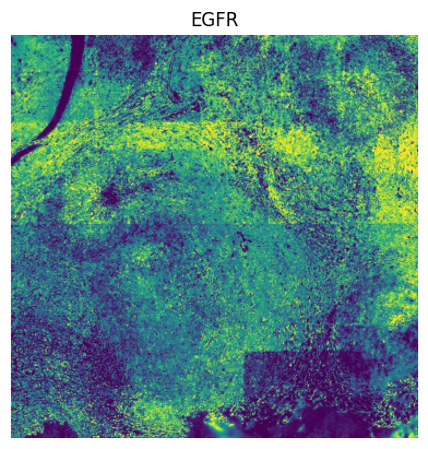
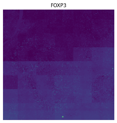
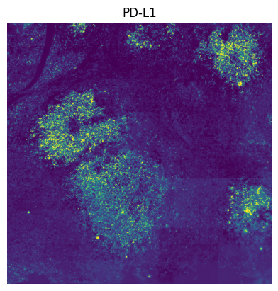
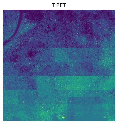
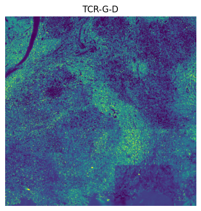
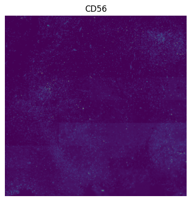
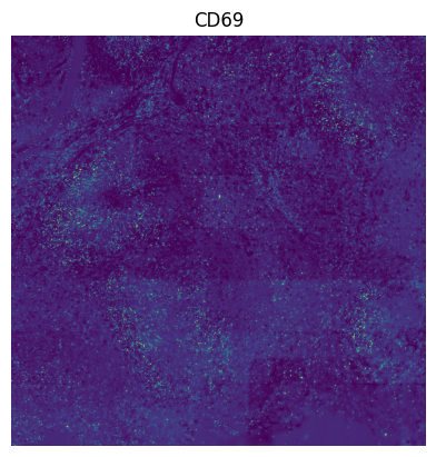
# We do leiden clustering with these channels filtered out: [ "EGFR", "FOXP3", "PD-L1", "T-BET", "TCR-G-D", "CD56", "CD69" ], because there are tiling effects in them.
subset_channels = [
_channel
for _channel in sdata[f"{table_name}_normalized"].var_names
if _channel not in ["EGFR", "FOXP3", "PD-L1", "T-BET", "TCR-G-D", "CD56", "CD69"]
]
sdata = hp.tb.leiden(
sdata,
labels_name="segmentation_mask",
table_name=f"{table_name}_normalized",
output_table_name=f"{table_name}_normalized_leiden", # write to new slot, because we subset the channels
index_names_var=subset_channels,
key_added="leiden",
overwrite=True,
)
sdata[f"{table_name}_normalized"].to_df().head()
| channels | BCL-2 | CCR6 | CD11B | CD11C | CD15 | CD16 | CD162 | CD163 | CD2 | CD20 | ... | PD-L1 | PODOPLANIN | T-BET | TCR-G-D | TCRB | TIM-3 | VISA | VIMENTIN | A-SMA | B-CATENIN |
|---|---|---|---|---|---|---|---|---|---|---|---|---|---|---|---|---|---|---|---|---|---|
| cells | |||||||||||||||||||||
| 1_segmentation_mask_3314222a | 79.668221 | 62.177567 | 0.011111 | 0.004568 | 0.003408 | 14.284677 | 0.796612 | 1.115642 | 36.489056 | 100.000000 | ... | 8.457295 | 11.425946 | 24.895376 | 68.573784 | 16.188705 | 0.666807 | 0.045563 | 13.841380 | 4.506205 | 5.740132 |
| 2_segmentation_mask_3314222a | 0.000000 | 12.825038 | 25.464931 | 66.745941 | 4.445347 | 0.540707 | 17.625029 | 1.495494 | 0.159467 | 0.000900 | ... | 15.119448 | 0.019308 | 1.770379 | 23.398777 | 5.933077 | 11.275876 | 18.348717 | 86.695709 | 2.516554 | 26.469042 |
| 3_segmentation_mask_3314222a | 6.095829 | 13.564084 | 29.563736 | 10.116818 | 10.844443 | 14.215184 | 0.021406 | 1.119725 | 0.428128 | 2.274806 | ... | 15.800408 | 0.019308 | 4.089499 | 20.374371 | 0.000000 | 0.505222 | 45.614468 | 7.071009 | 5.945360 | 10.390767 |
| 4_segmentation_mask_3314222a | 0.000581 | 1.295561 | 26.615061 | 21.340773 | 0.001544 | 9.267047 | 1.713156 | 29.938982 | 7.861145 | 0.002181 | ... | 4.889379 | 0.601552 | 0.454439 | 0.000000 | 5.325017 | 14.963484 | 22.917997 | 5.573087 | 100.000000 | 28.040024 |
| 5_segmentation_mask_3314222a | 20.208799 | 11.138199 | 0.011111 | 0.962152 | 0.003408 | 0.546169 | 75.941795 | 1.660741 | 33.755424 | 5.957442 | ... | 2.496632 | 1.173647 | 13.206595 | 15.744198 | 60.711853 | 1.350131 | 0.044816 | 22.877638 | 30.019194 | 0.000000 |
5 rows × 49 columns
table_name
'table_intensities'
Add the calculated leiden cluster ids to the table element where we did not subset the channels. This allows us to calculate mean intensity on all channels layer on.
import pandas as pd

from spatialdata.models import TableModel

instance_key = sdata[table_name].uns[TableModel.ATTRS_KEY][TableModel.INSTANCE_KEY]
region_key = sdata[table_name].uns[TableModel.ATTRS_KEY][TableModel.REGION_KEY_KEY]

index = sdata[f"{table_name}_normalized"].obs.index
name = sdata[f"{table_name}_normalized"].obs.index.name

if "leiden" in sdata[f"{table_name}_normalized"].obs.columns:
    sdata[f"{table_name}_normalized"].obs.drop(columns=["leiden"], inplace=True)

sdata[f"{table_name}_normalized"].obs = pd.merge(
    sdata[f"{table_name}_normalized"].obs,
    sdata[f"{table_name}_normalized_leiden"].obs[["leiden", region_key, instance_key]],
    on=[instance_key, region_key],
    how="inner",
)
sdata[f"{table_name}_normalized"].obs.index = index
sdata[f"{table_name}_normalized"].obs.index.name = name

# back to zarr store
sdata = hp.tb.add_table(
    sdata,
    adata=sdata[f"{table_name}_normalized"],
    output_table_name=f"{table_name}_normalized",
    region=["segmentation_mask"],
    overwrite=True,
)
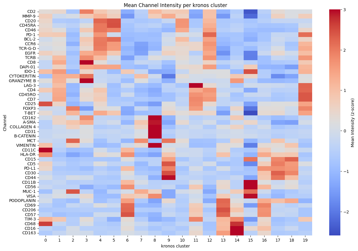
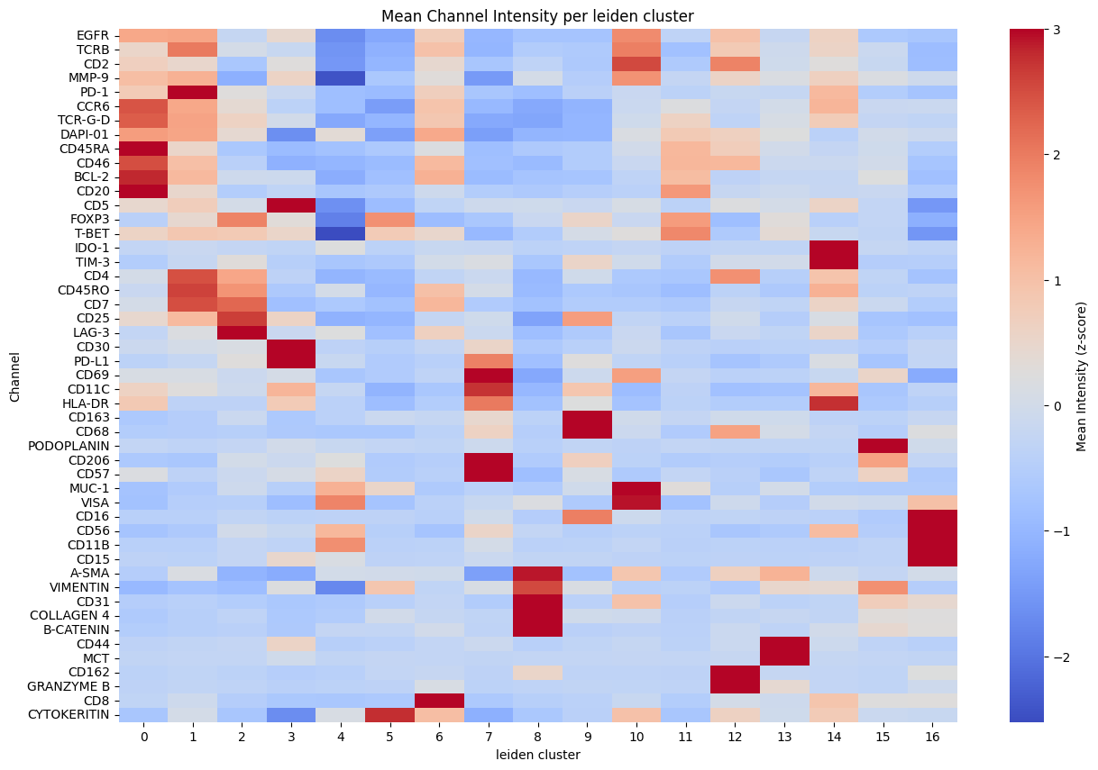
for _cluster in ["kronos", "leiden"]:
    sdata = hp.tb.cluster_intensity(
        sdata,
        table_name=f"{table_name}_normalized",
        labels_name="segmentation_mask",
        output_table_name=f"{table_name}_normalized",
        cluster_key=_cluster,
        layer_mean_intensities="raw_counts",  # layer in adata.layers that holds the mean intensities
        overwrite=True,
    )
    hp.pl.cluster_intensity_heatmap(
        sdata,
        table_name=f"{table_name}_normalized",
        cluster_key=_cluster,
        figsize=(15, 10),
    )
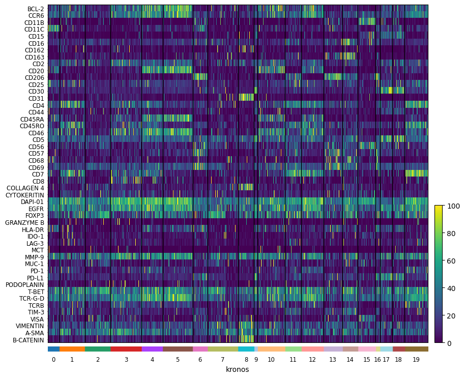
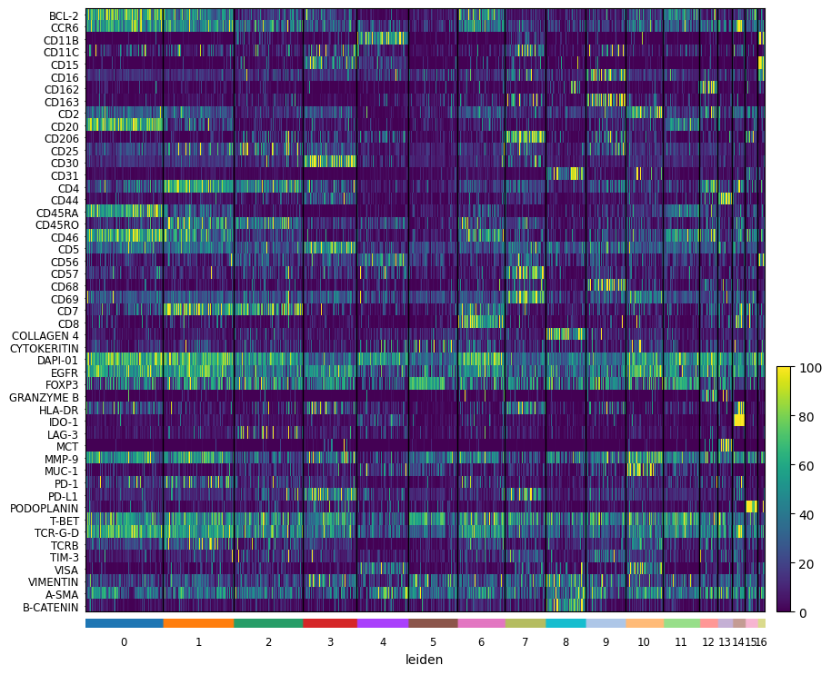
import scanpy as sc
from matplotlib.colors import Normalize

norm = Normalize(vmax=100, clip=False)
sc.pl.heatmap(
    sdata[f"{table_name}_normalized"],
    var_names=sdata[f"{table_name}_normalized"].var_names,
    groupby="kronos",
    swap_axes=True,
    norm=norm,
    use_raw=False,
)

sc.pl.heatmap(
    sdata[f"{table_name}_normalized"],
    var_names=sdata[f"{table_name}_normalized"].var_names,
    groupby="leiden",
    swap_axes=True,
    norm=norm,
    use_raw=False,
)
sdata[f"{table_name}_normalized"].obsm["X_umap"] = sdata[f"{table_name}_normalized_leiden"].obsm["X_umap"]
import scanpy as sc
from matplotlib.colors import Normalize
sc.pl.umap(sdata[f"{table_name}_normalized"], color=["cell_type"])
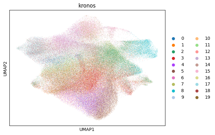
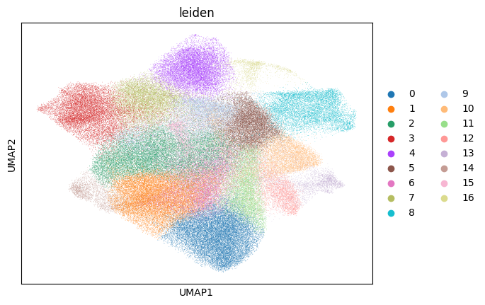
for _cluster_key in ["kronos", "leiden"]:
sc.pl.umap(sdata[f"{table_name}_normalized"], color=[_cluster_key])
norm = Normalize(vmax=100, clip=False)
sc.pl.umap(
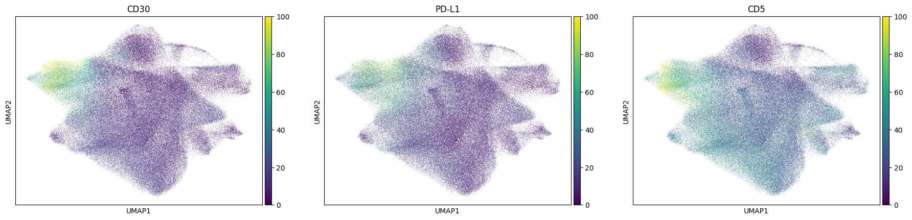
sdata[f"{table_name}_normalized"], color=["CD30", "PD-L1", "CD5"], norm=norm, use_raw=False
) # tumor markers
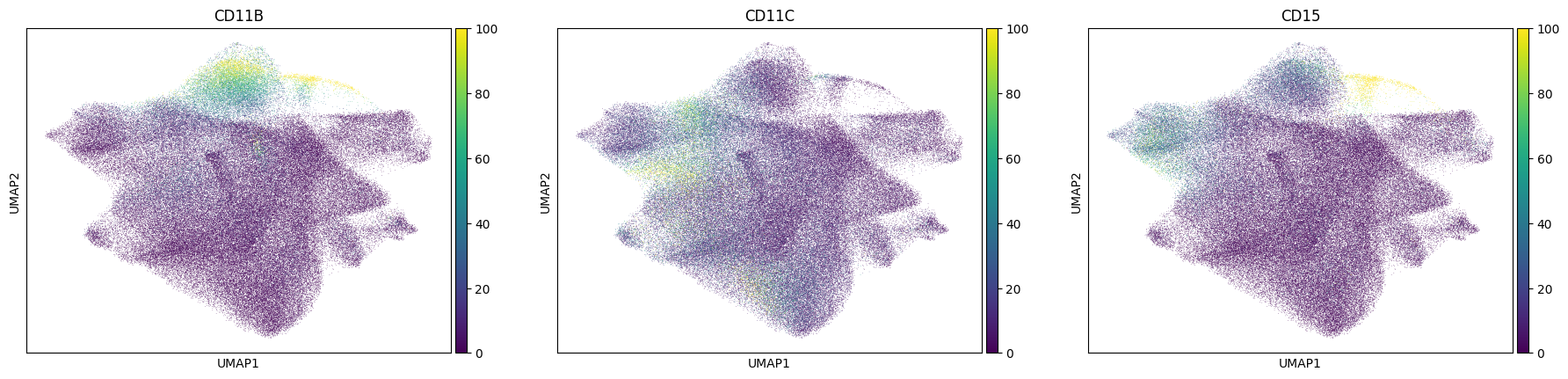
sc.pl.umap(sdata[f"{table_name}_normalized"], color=["CD11B", "CD11C", "CD15"], norm=norm, use_raw=False)
# note that these umaps are biased towards the leiden clusters (clusters will look more spatially seperated), because umaps are calculated on the same knn graph as the leiden clusters.
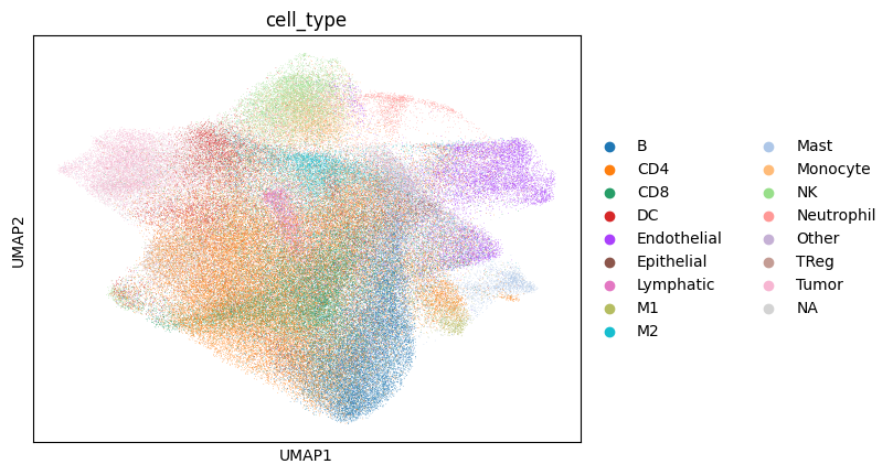
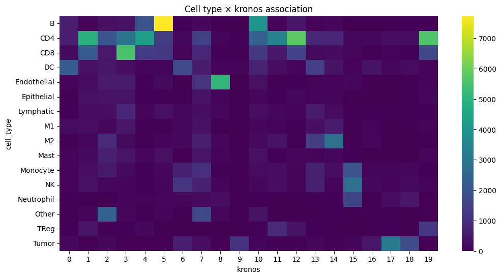
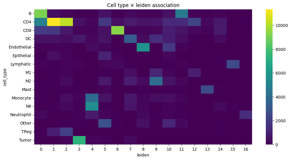
Next we try to estimate the measure of association between the KRONOS/Leiden clusters and the annotated cell type, by calculating the Cramers V statistic.
import matplotlib.pyplot as plt
import numpy as np
import pandas as pd
import seaborn as sns
from scipy.stats import chi2_contingency
for _cluster_key in ["kronos", "leiden"]:
df = sdata[f"{table_name}_normalized"].obs
df = df[~df["cell_type_id"].isna()]
contingency = pd.crosstab(df["cell_type"], df[_cluster_key])
# chi squared test
chi2, p, dof, expected = chi2_contingency(contingency)
# cramers v
def _cramers_v(confusion_matrix):
chi2 = chi2_contingency(confusion_matrix)[0]
n = confusion_matrix.sum().sum()
phi2 = chi2 / n
r, k = confusion_matrix.shape
return np.sqrt(phi2 / min(k - 1, r - 1))
print("Cramers v:", _cramers_v(contingency))
print("Chi-squared statistic:", chi2)
print("p-value:", p)
plt.figure(figsize=(12, 6))
sns.heatmap(contingency, cmap="viridis")
plt.title(f"Cell type × {_cluster_key} association")
plt.show()
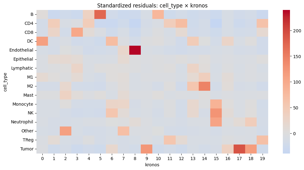
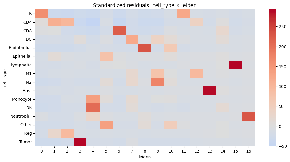
# Calculate standardized residuals
residuals = (contingency - expected) / np.sqrt(expected)
residuals_df = pd.DataFrame(residuals, index=contingency.index, columns=contingency.columns)
resid_long = residuals_df.stack().reset_index()
resid_long.columns = ["cell_type", _cluster_key, "std_residual"]
# Sort by strength of deviation
resid_long["abs_resid"] = resid_long["std_residual"].abs()
top_effects = resid_long.sort_values("abs_resid", ascending=False).head(20)
print(top_effects)
plt.figure(figsize=(12, 6))
sns.heatmap(residuals_df, center=0, cmap="coolwarm", annot=False)
plt.title(f"Standardized residuals: cell_type × {_cluster_key}")
plt.show()
Cramers v: 0.40833263281018034
Chi-squared statistic: 359473.4853451965
p-value: 0.0
       cell_type kronos  std_residual   abs_resid
88   Endothelial      8    239.920615  239.920615
317        Tumor     17    190.376840  190.376840
5              B      5    173.119357  173.119357
174           M2     14    143.902390  143.902390
235           NK     15    125.539999  125.539999
309        Tumor      9    122.268829  122.268829
318        Tumor     18    114.545215  114.545215
262        Other      2    112.218924  112.218924
60            DC      0    110.584902  110.584902
255   Neutrophil     15    108.023549  108.023549
43           CD8      3    101.712499  101.712499
215     Monocyte     15     87.373576   87.373576
10             B     10     80.813422   80.813422
32           CD4     12     72.044409   72.044409
66            DC      6     72.007998   72.007998
267        Other      7     68.878832   68.878832
299         TReg     19     67.417829   67.417829
39           CD4     19     64.061963   64.061963
173           M2     13     57.987977   57.987977
226           NK      6     57.130258   57.130258
Cramers v: 0.573074536541328
Chi-squared statistic: 708045.0783542951
p-value: 0.0
       cell_type leiden  std_residual   abs_resid
258        Tumor      3    292.654256  292.654256
117    Lymphatic     15    291.562718  291.562718
166         Mast     13    289.693060  289.693060
76   Endothelial      8    231.233794  231.233794
220   Neutrophil     16    228.920163  228.920163
40           CD8      6    222.583909  222.583909
191           NK      4    203.898082  203.898082
145           M2      9    175.362353  175.362353
0              B      0    160.610434  160.610434
174     Monocyte      4    139.437011  139.437011
226        Other      5    134.999515  134.999515
11             B     11    124.371550  124.371550
58            DC      7    122.938085  122.938085
18           CD4      1    112.172448  112.172448
19           CD4      2     98.468486   98.468486
131           M1     12     94.287696   94.287696
240         TReg      2     93.462668   93.462668
90    Epithelial      5     77.534145   77.534145
128           M1      9     74.155199   74.155199
78   Endothelial     10     59.498226   59.498226
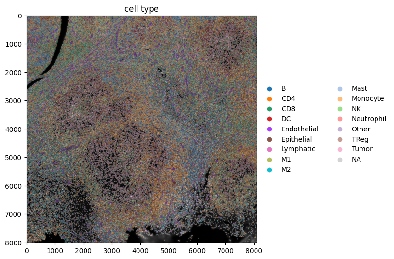
Next, we spatially plot the KRONOS and Leiden clusters, and the cell types.
import dask.array as da
import matplotlib.pyplot as plt
import numpy as np
from matplotlib.colors import Normalize


c = "DAPI-01"

table_name = f"{table_name}_normalized"

se = hp.im.get_dataarray(sdata, element_name="image")
channels = se.c.data

c_id = np.where(channels == c)[0].item()
vmax = da.percentile(se.data[c_id].flatten(), q=99).compute()  # clip to 99% percentile
norm = Normalize(vmax=vmax, clip=True)

render_images_kwargs = {
    "cmap": "grey",
    "norm": norm,
    "scale": "scale3",
}
render_labels_kwargs = {
    "scale": "scale2",
    "fill_alpha": 0.2,
    "outline_alpha": 0.3,
}

show_kwargs = {"title": "kronos", "colorbar": False, "dpi": 100, "figsize": (8, 8)}
ax = hp.pl.plot_sdata(
    sdata,
    ax=None,
    image_name="image",
    channel=c,
    labels_name="segmentation_mask",
    table_name=table_name,
    color="kronos",
    render_images_kwargs=render_images_kwargs,
    render_labels_kwargs=render_labels_kwargs,
    show_kwargs=show_kwargs,
)

show_kwargs = {"title": "leiden", "colorbar": False, "dpi": 100, "figsize": (8, 8)}
ax = hp.pl.plot_sdata(
    sdata,
    ax=None,
    image_name="image",
    channel=c,
    labels_name="segmentation_mask",
    table_name=table_name,
    color="leiden",
    render_images_kwargs=render_images_kwargs,
    render_labels_kwargs=render_labels_kwargs,
    show_kwargs=show_kwargs,
)

show_kwargs = {"title": "cell type", "colorbar": False, "dpi": 100, "figsize": (8, 8)}
ax = hp.pl.plot_sdata(
    sdata,
    ax=None,
    image_name="image",
    channel=c,
    labels_name="segmentation_mask",
    table_name=table_name,
    color="cell_type",
    render_images_kwargs=render_images_kwargs,
    render_labels_kwargs=render_labels_kwargs,
    show_kwargs=show_kwargs,
)
INFO     Rasterizing image for faster rendering.
INFO     Rasterizing image for faster rendering.
INFO     Rasterizing image for faster rendering.
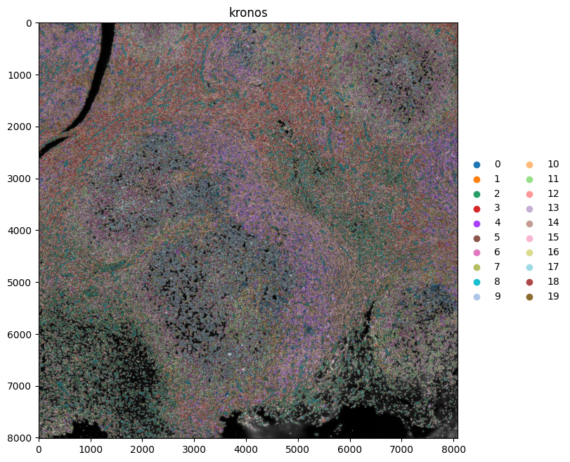
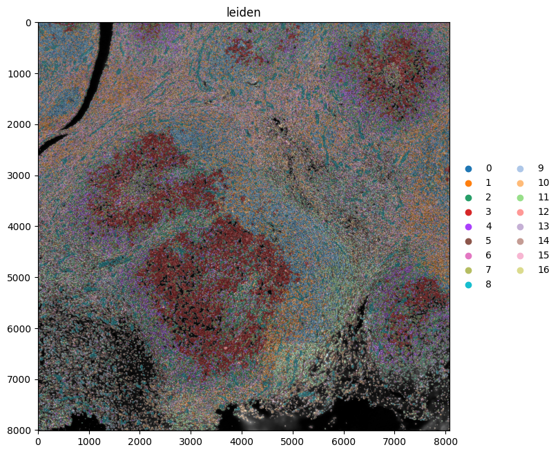
The tiling effects in the leiden clusters are caused by the tiling effects visible in some of the channels. By removing the channels “EGFR”, “FOXP3”, “PD-L1”, “T-BET”, “TCR-G-D”, “CD56” and “CD69”, a lot of the tiling effects were removed when spatially plotting the leiden clusters.
Note that when plotting the kronos clusters spatially, such tiling effects are not observed.
norm = Normalize(vmin=0, vmax=10000, clip=True)

render_images_kwargs = {
    "cmap": "viridis",
    "norm": norm,
    "scale": "scale3",
}

for channel in [
    "EGFR",
    "FOXP3",
    "PD-L1",
    "T-BET",
    "TCR-G-D",
    "CD56",
    "CD69",
]:  # these channels causing tiling artefact in leiden clustering.
    show_kwargs = {"title": str(channel), "colorbar": False, "dpi": 100, "figsize": (4, 4)}

    ax = hp.pl.plot_sdata(
        sdata,
        ax=None,
        image_name="image",
        channel=channel,
        render_images_kwargs=render_images_kwargs,
        show_kwargs=show_kwargs,
    )
    ax.axis("off")