Working with multiple samples (and coordinate systems)

In this notebook, we will work with mouse liver spatial transcriptomics data generated using Resolve Biosciences’ Molecular Cartography technology, to illustrate the use of multiple samples and coordinate systems in Harpy and SpatialData.

1. Read the images into a SpatialData object backed by a zarr store.

import os

import tempfile
import uuid

from spatialdata import SpatialData

import harpy as hp

sdata = SpatialData()

default_tmp_path = tempfile.gettempdir()

zarr_path = os.path.join(default_tmp_path, f"sdata_{uuid.uuid4()}.zarr")

sdata.write(zarr_path)

Add image elements.

from dask_image import imread
from spatialdata.transformations import Identity, Scale

from harpy.datasets.registry import get_registry

registry = get_registry()
arr_a1_1 = imread.imread(registry.fetch("transcriptomics/resolve/mouse/20272_slide1_A1-1_DAPI.tiff"))
arr_a1_2 = imread.imread(registry.fetch("transcriptomics/resolve/mouse/20272_slide1_A1-2_DAPI.tiff"))

pixel_size = 0.138  # pixel size in micron for resolve
scale = Scale(axes=["x", "y"], scale=[pixel_size, pixel_size])

sdata = hp.im.add_image(
    sdata,
    arr=arr_a1_1,
    output_image_name="image_a1_1",
    transformations={"a1_1_pixel": Identity(), "a1_1_micron": scale},
    c_coords="DAPI",
    scale_factors=[2, 2, 2, 2],
    overwrite=True,
)

sdata = hp.im.add_image(
    sdata,
    arr=arr_a1_2,
    output_image_name="image_a1_2",
    transformations={"a1_2_pixel": Identity(), "a1_2_micron": scale},
    c_coords="DAPI",
    scale_factors=[2, 2, 2, 2],
    overwrite=True,
)

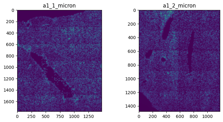
2. Specify coordinate system when plotting.

import matplotlib.pyplot as plt

fig, axes = plt.subplots(1, 2, figsize=(8, 4))

channel = "DAPI"
render_images_kwargs = {
    "cmap": "viridis",
}

image_name = ["image_a1_1", "image_a1_2"]
to_coordinate_system = ["a1_1_micron", "a1_2_micron"]

for _image_name, _to_coordinate_system, _ax in zip(image_name, to_coordinate_system, axes, strict=True):
    show_kwargs = {"title": _to_coordinate_system, "colorbar": False}
    _ax = hp.pl.plot_sdata(
        sdata,
        image_name=_image_name,
        channel=channel,
        crd=None,
        to_coordinate_system=_to_coordinate_system,
        render_images_kwargs=render_images_kwargs,
        show_kwargs=show_kwargs,
        ax=_ax,
    )

plt.tight_layout()
plt.show()

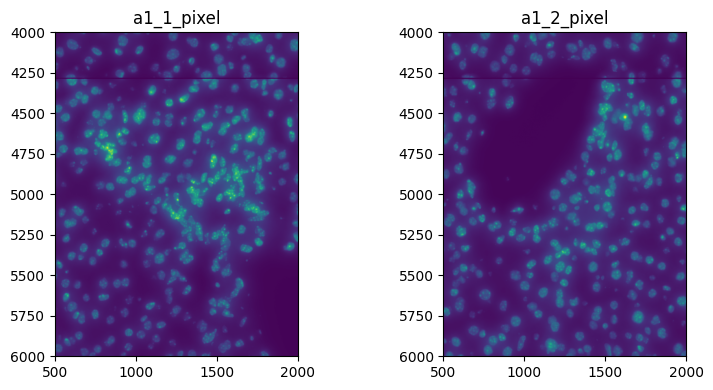
Visualize a crop:

import matplotlib.pyplot as plt

fig, axes = plt.subplots(1, 2, figsize=(8, 4))

channel = "DAPI"
render_images_kwargs = {
    "cmap": "viridis",
}

image_name = ["image_a1_1", "image_a1_2"]
to_coordinate_system = ["a1_1_pixel", "a1_2_pixel"]

for _image_name, _to_coordinate_system, _ax in zip(image_name, to_coordinate_system, axes, strict=True):
    show_kwargs = {"title": _to_coordinate_system, "colorbar": False}
    _ax = hp.pl.plot_sdata(
        sdata,
        image_name=_image_name,
        channel=channel,
        crd=[500, 2000, 4000, 6000],
        to_coordinate_system=_to_coordinate_system,
        render_images_kwargs=render_images_kwargs,
        show_kwargs=show_kwargs,
        ax=_ax,
    )

plt.tight_layout()
plt.show()

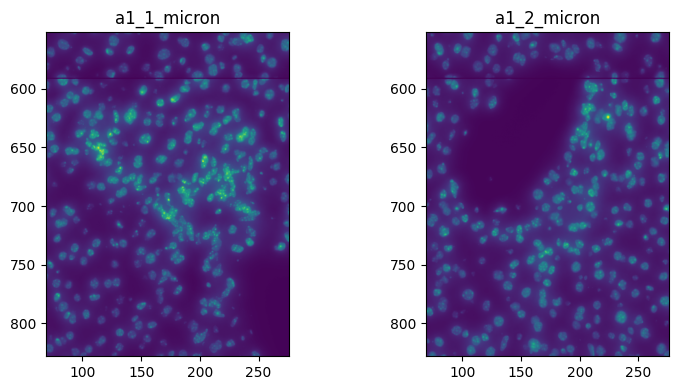
Or in micron

import matplotlib.pyplot as plt

fig, axes = plt.subplots(1, 2, figsize=(8, 4))

channel = "DAPI"
render_images_kwargs = {
    "cmap": "viridis",
}

image_name = ["image_a1_1", "image_a1_2"]
to_coordinate_system = ["a1_1_micron", "a1_2_micron"]

for _image_name, _to_coordinate_system, _ax in zip(image_name, to_coordinate_system, axes, strict=True):
    show_kwargs = {"title": _to_coordinate_system, "colorbar": False}
    _ax = hp.pl.plot_sdata(
        sdata,
        image_name=_image_name,
        channel=channel,
        crd=[69, 276, 552, 828],
        to_coordinate_system=_to_coordinate_system,
        render_images_kwargs=render_images_kwargs,
        show_kwargs=show_kwargs,
        ax=_ax,
    )

plt.tight_layout()
plt.show()

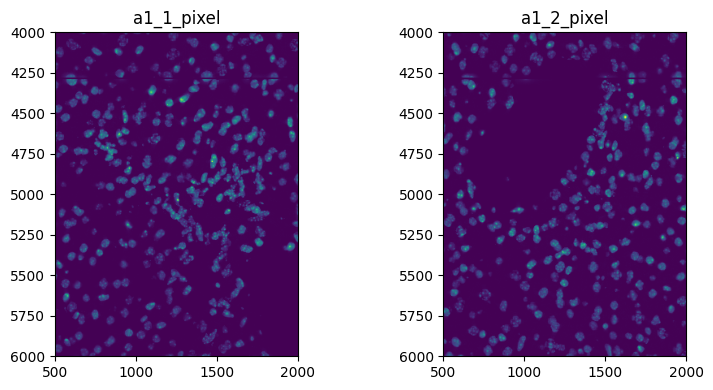
3. Image processing.

Do some image processing on the full image, no need to specify a coordinate system

sdata = hp.im.min_max_filtering(
    sdata, image_name="image_a1_1", output_image_name="image_a1_1_min_max", size_min_max_filter=40, overwrite=True
)

When doing some image processing on a crop, you need to specify the coordinate system to which the crop is defined

for image_name, to_coordinate_system in zip(["image_a1_1", "image_a1_2"], ["a1_1_pixel", "a1_2_pixel"], strict=True):
    sdata = hp.im.min_max_filtering(
        sdata,
        image_name=image_name,
        output_image_name=f"{image_name}_min_max",
        size_min_max_filter=40,
        crd=[500, 2000, 4000, 6000],
        to_coordinate_system=to_coordinate_system,
        overwrite=True,
    )

fig, axes = plt.subplots(1, 2, figsize=(8, 4))

channel = "DAPI"
render_images_kwargs = {
    "cmap": "viridis",
}

for image_name, to_coordinate_system, ax in zip(
    ["image_a1_1_min_max", "image_a1_2_min_max"], ["a1_1_pixel", "a1_2_pixel"], axes, strict=True
):
    show_kwargs = {"title": to_coordinate_system, "colorbar": False}
    ax = hp.pl.plot_sdata(
        sdata,
        image_name=image_name,
        channel=channel,
        crd=None,
        to_coordinate_system=to_coordinate_system,
        render_images_kwargs=render_images_kwargs,
        show_kwargs=show_kwargs,
        ax=ax,
    )

plt.tight_layout()
plt.show()

INFO     Rasterizing image for faster rendering.                                                                   
INFO     Rasterizing image for faster rendering.

4. Segmentation.

# no need to specify coordinate system if no crop is specifed
import torch
from dask.distributed import LocalCluster, Client

cluster = LocalCluster(
    n_workers=1
    if torch.backends.mps.is_available() or torch.cuda.is_available()
    else 8,  # If mps/cuda device available, it is better to increase chunk size to maximal value that fits on the gpu, and set n_workers to 1.
    threads_per_worker=1,
    memory_limit="32GB",
    # local_directory=os.environ.get( "TMPDIR" ),
)

client = Client(cluster)

print(client.dashboard_link)

sdata = hp.im.segment(
    sdata,
    image_name="image_a1_1_min_max",
    output_labels_name="labels_a1_1",
    output_shapes_name="shapes_a1_1",
    overwrite=True,
    crd=None,
)

# but need to specify coordinate system when crop is defined

sdata = hp.im.segment(
    sdata,
    image_name="image_a1_2_min_max",
    output_labels_name="labels_a1_2",
    output_shapes_name="shapes_a1_2",
    overwrite=True,
    crd=[600, 2000, 4000, 6000],
    to_coordinate_system="a1_2_pixel",
)
client.close()

http://127.0.0.1:64440/status

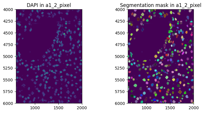
fig, axes = plt.subplots(1, 2, figsize=(8, 4))

channel = "DAPI"
image_name = "image_a1_2_min_max"
labels_name = "labels_a1_2"
crd = [600, 2000, 4000, 6000]  # Crop in pixels. One could also choose to do the crop in micron coordinates
to_coordinate_system = "a1_2_pixel"

render_images_kwargs = {"cmap": "viridis"}
render_labels_kwargs = {"fill_alpha": 0.6, "outline_alpha": 0.4}
show_kwargs = {"title": f"DAPI in {to_coordinate_system}", "colorbar": False}

_ax = hp.pl.plot_sdata(
    sdata,
    image_name=image_name,
    crd=crd,
    to_coordinate_system=to_coordinate_system,
    channel=channel,
    render_images_kwargs=render_images_kwargs,
    show_kwargs=show_kwargs,
    ax=axes[0],
)
# _ax.axis("off")

show_kwargs = {"title": f"Segmentation mask in {to_coordinate_system}", "colorbar": False}
_ax = hp.pl.plot_sdata(
    sdata,
    image_name=image_name,
    labels_name=labels_name,
    crd=crd,
    to_coordinate_system=to_coordinate_system,
    channel=channel,
    render_images_kwargs=render_images_kwargs,
    render_labels_kwargs=render_labels_kwargs,
    show_kwargs=show_kwargs,
    ax=axes[1],
)
# _ax.axis("off")

plt.tight_layout()
plt.show()

INFO     Rasterizing image for faster rendering.                                                                   
INFO     Rasterizing image for faster rendering.                                                                   
INFO     Rasterizing image for faster rendering.

Read the transcripts downloaded previously. For downstream analysis it is convenient if the transcripts are stored in pixels (intrinsic coordinate system of the images), and registered with the images. Therefore, if transcripts are delivered in micron, it is possible to specify an affine transformation via the parameter transform_matrix of the function harpy.io.read_transcripts that converts from micron to pixels, and registers the transcripts with the images. A micron coordinate system will be added to the resulting points element of the SpatialData object if to_micron_coordinate_system is specified. We refer to the docstring of harpy.io.read_transcripts for more information.

Transcripts from Resolve Biosciences’ Molecular Cartography technology are already in pixels. By specifying the pixel size and the micron coordinate system, the function harpy.io.read_transcripts takes care of adding a micron coordinate system.

path_transcripts_a1_1 = registry.fetch("transcriptomics/resolve/mouse/20272_slide1_A1-1_results.txt")
path_transcripts_a1_2 = registry.fetch("transcriptomics/resolve/mouse/20272_slide1_A1-2_results.txt")

sdata = hp.io.read_transcripts(
    sdata,
    path_count_matrix=path_transcripts_a1_1,
    column_x=0,
    column_y=1,
    column_gene=3,
    delimiter="\t",
    header=None,
    output_points_name="transcripts_a1_1",
    to_coordinate_system="a1_1_pixel",
    to_micron_coordinate_system="a1_1_micron",
    pixel_size=pixel_size,  # size of pixels in micron
    transform_matrix=None,  # transcripts are already in pixels, and registered with the images
    overwrite=True,
)

sdata = hp.io.read_transcripts(
    sdata,
    path_count_matrix=path_transcripts_a1_2,
    column_x=0,
    column_y=1,
    column_gene=3,
    delimiter="\t",
    header=None,
    output_points_name="transcripts_a1_2",
    to_coordinate_system="a1_2_pixel",
    to_micron_coordinate_system="a1_2_micron",
    pixel_size=pixel_size,  # size of pixels in micron
    transform_matrix=None,  # transcripts are already in pixels, and registered with the images
    overwrite=True,
)

Verify that transformation associated to points element in the pixel coordinate system is indeed the identity, and verify that the labels have same transformation associated to them.

from spatialdata.transformations import get_transformation

print(
    f"points:\n {get_transformation(sdata['transcripts_a1_2'], to_coordinate_system='a1_2_pixel')}\n",
)
print(
    f"image:\n{get_transformation(sdata['image_a1_2_min_max'], to_coordinate_system='a1_2_pixel')}\n",
)  # one crop was taken, so an extra translation is defined on image.
print(
    f"image:\n{get_transformation(sdata['labels_a1_2'], to_coordinate_system='a1_2_pixel')}\n",
)  # two times a crop was taken, so a sequence of two translations is defined on labels and the associated shapes.
print(
    f"shapes:\n{get_transformation(sdata['shapes_a1_2'], to_coordinate_system='a1_2_pixel')}\n",
)  # two times a crop was taken, so a sequence of two translations is defined on labels and the associated shapes.

points:
 Identity 

image:
Sequence 
    Translation (c, y, x)
        [   0. 4000.  500.]
    Identity 

image:
Sequence 
    Translation (y, x)
        [  0. 100.]
    Sequence 
        Translation (y, x)
            [4000.  500.]
        Identity 

shapes:
Sequence 
    Translation (x, y)
        [100.   0.]
    Sequence 
        Translation (x, y)
            [ 500. 4000.]
        Identity

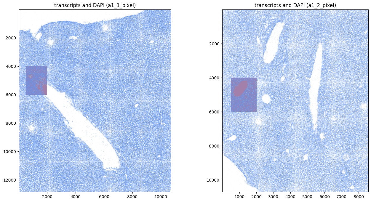
fig, axes = plt.subplots(1, 2, figsize=(16, 8))

render_images_kwargs = {
    "cmap": "viridis",
    "alpha": 0.5,
}

image_name = ["image_a1_1_min_max", "image_a1_2_min_max"]
points_name = ["transcripts_a1_1", "transcripts_a1_2"]
to_coordinate_system = ["a1_1_pixel", "a1_2_pixel"]

for _image_name, _points_name, _to_coordinate_system, _ax in zip(
    image_name, points_name, to_coordinate_system, axes, strict=True
):
    show_kwargs = {
        "title": f"transcripts and DAPI ({_to_coordinate_system})",
        "colorbar": False,
    }

    hp.pl.plot_sdata_genes(
        sdata,
        points_name=_points_name,
        image_name=_image_name,
        genes=None,  # plot all genes
        color="cornflowerblue",
        size=0.1,
        frac=0.5,  # only plot half of them
        to_coordinate_system=_to_coordinate_system,
        show_kwargs=show_kwargs,
        render_images_kwargs=render_images_kwargs,
        ax=_ax,
    )

INFO     Value for parameter 'color' appears to be a color, using it as such.                                      
INFO     Rasterizing image for faster rendering.
INFO     Using 'datashader' backend with 'None' as reduction method to speed up plotting. Depending on the         
         reduction method, the value range of the plot might change. Set method to 'matplotlib' do disable this    
         behaviour.
INFO     Value for parameter 'color' appears to be a color, using it as such.                                      
INFO     Rasterizing image for faster rendering.
INFO     Using 'datashader' backend with 'None' as reduction method to speed up plotting. Depending on the         
         reduction method, the value range of the plot might change. Set method to 'matplotlib' do disable this    
         behaviour.

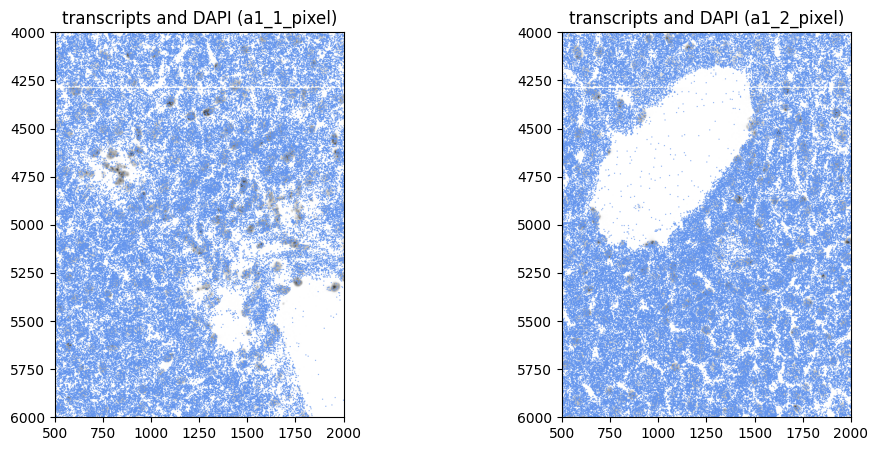
Or visualize a crop:

# we query the points elements outside of spatialdata, because querying points via spatialdata.bounding_box_query is slow

crd = [500, 2000, 4000, 6000]

points_name = ["transcripts_a1_1", "transcripts_a1_2"]

to_coordinate_system = ["a1_1_pixel", "a1_2_pixel"]

for _points_name, _to_coordinate_system in zip(points_name, to_coordinate_system, strict=True):
    to_coordinate_system = _to_coordinate_system  # we query in 'intrinsic' pixel coordinate system

    y_start = crd[2]
    x_start = crd[0]

    y_end = crd[3]
    x_end = crd[1]

    name_x = "x"
    name_y = "y"

    y_query = f"{y_start} <={name_y} < {y_end}"
    x_query = f"{x_start} <={name_x} < {x_end}"

    query = f"{y_query} and {x_query}"

    sdata[f"{_points_name}_queried"] = sdata[_points_name].query(query)


fig, axes = plt.subplots(1, 2, figsize=(12, 5))

render_images_kwargs = {
    "cmap": "binary",
}

image_name = ["image_a1_1_min_max", "image_a1_2_min_max"]
points_name = [f"{_points_name}_queried" for _points_name in points_name]
to_coordinate_system = ["a1_1_pixel", "a1_2_pixel"]

for _image_name, _points_name, _to_coordinate_system, _ax in zip(
    image_name, points_name, to_coordinate_system, axes, strict=True
):
    show_kwargs = {
        "title": f"transcripts and DAPI ({_to_coordinate_system})",
        "colorbar": False,
    }

    hp.pl.plot_sdata_genes(
        sdata,
        points_name=_points_name,
        image_name=_image_name,
        genes=None,  # plot all genes
        color="cornflowerblue",
        size=1,
        frac=None,  # only plot half of them
        to_coordinate_system=_to_coordinate_system,
        show_kwargs=show_kwargs,
        render_images_kwargs=render_images_kwargs,
        ax=_ax,
    )

    del sdata[_points_name]

INFO     Value for parameter 'color' appears to be a color, using it as such.                                      
INFO     Rasterizing image for faster rendering.                                                                   
INFO     Using 'datashader' backend with 'None' as reduction method to speed up plotting. Depending on the         
         reduction method, the value range of the plot might change. Set method to 'matplotlib' do disable this    
         behaviour.
INFO     Value for parameter 'color' appears to be a color, using it as such.                                      
INFO     Rasterizing image for faster rendering.                                                                   
INFO     Using 'datashader' backend with 'None' as reduction method to speed up plotting. Depending on the         
         reduction method, the value range of the plot might change. Set method to 'matplotlib' do disable this    
         behaviour.

5. Create the AnnData table.

# Use dask cluster for optimal processing. For this dummy example, one could also work without a dask cluster.
cluster = LocalCluster(
    n_workers=8,
    threads_per_worker=1,
    processes=True,
    memory_limit="8GB",
    # local_directory=os.environ.get( "TMPDIR" ),
)

client = Client(cluster)

print(client.dashboard_link)

sdata = hp.tb.allocate(
    sdata,
    labels_name="labels_a1_1",
    points_name="transcripts_a1_1",
    to_coordinate_system="a1_1_pixel",  # allocation step should always be run in pixel coordinates
    output_table_name="table",
    update_shapes_elements=False,
    append=False,
    overwrite=True,
)

# append gene count of labels_a1_2 and points_a1_2 to anndata object with name 'table'
sdata = hp.tb.allocate(
    sdata,
    labels_name="labels_a1_2",
    points_name="transcripts_a1_2",
    to_coordinate_system="a1_2_pixel",
    output_table_name="table",
    update_shapes_elements=False,
    append=True,
    overwrite=True,
)

client.close()

http://127.0.0.1:64454/status

from spatialdata.models import TableModel

print(sdata["table"].uns[TableModel.ATTRS_KEY], "\n")  # -> the table is annotated by "labels_a1_1" and "labels_a1_2"
print(
    sdata["table"].uns[TableModel.ATTRS_KEY][TableModel.REGION_KEY_KEY], "\n"
)  # -> column in .obs that holds the spatial element that is annotating the instance
print(
    sdata["table"].uns[TableModel.ATTRS_KEY][TableModel.INSTANCE_KEY]
)  # -> column in .obs that holds the instance id in the corresponding spatial element

{'region': ['labels_a1_1', 'labels_a1_2'], 'region_key': 'fov_labels', 'instance_key': 'cell_ID'} 

fov_labels 

cell_ID

display(sdata["table"].obs.head())
display(sdata["table"].obs.tail())

	cell_ID	fov_labels
cells
18_labels_a1_1_7f8836a8	18	labels_a1_1
19_labels_a1_1_7f8836a8	19	labels_a1_1
20_labels_a1_1_7f8836a8	20	labels_a1_1
21_labels_a1_1_7f8836a8	21	labels_a1_1
22_labels_a1_1_7f8836a8	22	labels_a1_1

	cell_ID	fov_labels
cells
346_labels_a1_2_caa1aa78	346	labels_a1_2
348_labels_a1_2_caa1aa78	348	labels_a1_2
349_labels_a1_2_caa1aa78	349	labels_a1_2
352_labels_a1_2_caa1aa78	352	labels_a1_2
353_labels_a1_2_caa1aa78	353	labels_a1_2

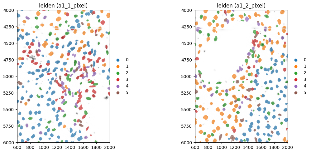
6. Leiden clustering.

sdata = hp.tb.preprocess_transcriptomics(
    sdata,
    labels_name=["labels_a1_1", "labels_a1_2"],
    table_name="table",
    output_table_name="table_preprocessed",
    update_shapes_elements=False,
    overwrite=True,
)  # we can also choose to set output_table_name equal to 'table'.

hp.tb.leiden(
    sdata,
    labels_name=["labels_a1_1", "labels_a1_2"],
    table_name="table_preprocessed",
    output_table_name="table_preprocessed",
    overwrite=True,
)

SpatialData object, with associated Zarr store: /private/var/folders/q5/7yhs0l6d0x771g7qdbhvkvmr0000gp/T/sdata_66a1e781-b62b-463e-b4be-ef244dc695ba.zarr
├── Images
│     ├── 'image_a1_1': DataTree[cyx] (1, 12864, 10720), (1, 6432, 5360), (1, 3216, 2680), (1, 1608, 1340), (1, 804, 670)
│     ├── 'image_a1_1_min_max': DataArray[cyx] (1, 2000, 1500)
│     ├── 'image_a1_2': DataTree[cyx] (1, 10720, 8576), (1, 5360, 4288), (1, 2680, 2144), (1, 1340, 1072), (1, 670, 536)
│     └── 'image_a1_2_min_max': DataArray[cyx] (1, 2000, 1500)
├── Labels
│     ├── 'labels_a1_1': DataArray[yx] (2000, 1500)
│     └── 'labels_a1_2': DataArray[yx] (2000, 1400)
├── Points
│     ├── 'transcripts_a1_1': DataFrame with shape: (<Delayed>, 3) (2D points)
│     └── 'transcripts_a1_2': DataFrame with shape: (<Delayed>, 3) (2D points)
├── Shapes
│     ├── 'shapes_a1_1': GeoDataFrame shape: (341, 1) (2D shapes)
│     └── 'shapes_a1_2': GeoDataFrame shape: (295, 1) (2D shapes)
└── Tables
      ├── 'table': AnnData (630, 88)
      └── 'table_preprocessed': AnnData (605, 78)
with coordinate systems:
    ▸ 'a1_1_micron', with elements:
        image_a1_1 (Images), image_a1_1_min_max (Images), labels_a1_1 (Labels), transcripts_a1_1 (Points), shapes_a1_1 (Shapes)
    ▸ 'a1_1_pixel', with elements:
        image_a1_1 (Images), image_a1_1_min_max (Images), labels_a1_1 (Labels), transcripts_a1_1 (Points), shapes_a1_1 (Shapes)
    ▸ 'a1_2_micron', with elements:
        image_a1_2 (Images), image_a1_2_min_max (Images), labels_a1_2 (Labels), transcripts_a1_2 (Points), shapes_a1_2 (Shapes)
    ▸ 'a1_2_pixel', with elements:
        image_a1_2 (Images), image_a1_2_min_max (Images), labels_a1_2 (Labels), transcripts_a1_2 (Points), shapes_a1_2 (Shapes)

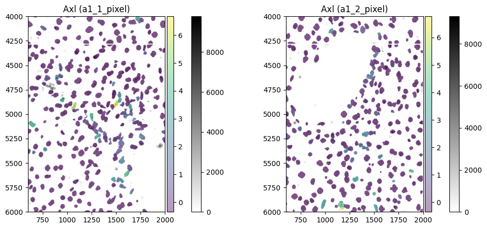
fig, axes = plt.subplots(1, 2, figsize=(12, 5))

channel = "DAPI"
image_name = ["image_a1_1_min_max", "image_a1_2_min_max"]
labels_name = ["labels_a1_1", "labels_a1_2"]
to_coordinate_system = ["a1_1_pixel", "a1_2_pixel"]
table_name = "table_preprocessed"

crd = [600, 2000, 4000, 6000]

render_images_kwargs = {"cmap": "binary"}
render_labels_kwargs = {"fill_alpha": 0.6, "outline_alpha": 0.4}

color = "Axl"

for _image_name, _labels_name, _to_coordinate_system, _ax in zip(
    image_name, labels_name, to_coordinate_system, axes, strict=True
):
    # subset because querying of points is slow, and we do not need them in this visualization

    sdata_to_plot = sdata.subset(element_names=[_image_name, _labels_name, table_name])

    show_kwargs = {
        "title": f"{color} ({_to_coordinate_system})",
        "colorbar": True,
    }
    _ax = hp.pl.plot_sdata(
        sdata_to_plot,
        image_name=_image_name,
        channel=channel,
        crd=crd,
        to_coordinate_system=_to_coordinate_system,
        labels_name=_labels_name,
        table_name=table_name,
        color=color,
        render_images_kwargs=render_images_kwargs,
        show_kwargs=show_kwargs,
        ax=_ax,
    )

fig, axes = plt.subplots(1, 2, figsize=(12, 5))

color = "leiden"

for _image_name, _labels_name, _to_coordinate_system, _ax in zip(
    image_name, labels_name, to_coordinate_system, axes, strict=True
):
    sdata_to_plot = sdata.subset(element_names=[_image_name, _labels_name, table_name])

    show_kwargs = {
        "title": f"{color} ({_to_coordinate_system})",
        "colorbar": False,
    }
    _ax = hp.pl.plot_sdata(
        sdata_to_plot,
        image_name=_image_name,
        channel=channel,
        crd=crd,
        to_coordinate_system=_to_coordinate_system,
        labels_name=_labels_name,
        table_name=table_name,
        color=color,
        render_images_kwargs=render_images_kwargs,
        show_kwargs=show_kwargs,
        ax=_ax,
    )

plt.tight_layout()
plt.show()

INFO     Rasterizing image for faster rendering.                                                                   
INFO     Rasterizing image for faster rendering.
INFO     Rasterizing image for faster rendering.                                                                   
INFO     Rasterizing image for faster rendering.
INFO     Rasterizing image for faster rendering.                                                                   
INFO     Rasterizing image for faster rendering.
INFO     Rasterizing image for faster rendering.                                                                   
INFO     Rasterizing image for faster rendering.

7. Query the labels elements and the associated table element it annotates.

zarr_path = os.path.join(default_tmp_path, f"sdata_{uuid.uuid4()}.zarr")  # output path for queried sdata

labels_name = [
    "labels_a1_1",
    "labels_a1_2",
]
crd = [
    (600, 1000, 4000, 5000),
    (700, 1000, 4000, 5000),
]  # queries could also be done in pixels
to_coordinate_system = ["a1_1_pixel", "a1_2_pixel"]

sdata_queried = hp.utils.bounding_box_query(
    sdata,
    labels_name=labels_name,
    crd=crd,
    to_coordinate_system=to_coordinate_system,
    copy_image=False,
    copy_shapes=False,
    copy_points=False,
    output=zarr_path,
)

for _labels_name in labels_name:
    assert _labels_name in sdata_queried.labels

from spatialdata.transformations import get_transformation

get_transformation(sdata_queried["labels_a1_1"], to_coordinate_system="a1_1_pixel")

Sequence 
    Translation (y, x)
        [  0. 100.]
    Sequence 
        Translation (y, x)
            [4000.  500.]
        Identity 

sdata_queried["table_preprocessed"]

AnnData object with n_obs × n_vars = 66 × 78
    obs: 'cell_ID', 'fov_labels', 'n_genes_by_counts', 'log1p_n_genes_by_counts', 'total_counts', 'log1p_total_counts', 'pct_counts_in_top_2_genes', 'pct_counts_in_top_5_genes', 'n_counts', 'shapeSize', 'leiden'
    var: 'n_cells_by_counts', 'mean_counts', 'log1p_mean_counts', 'pct_dropout_by_counts', 'total_counts', 'log1p_total_counts', 'n_cells', 'mean', 'std'
    uns: 'pca', 'spatialdata_attrs', 'umap', 'leiden', 'rank_genes_groups', 'log1p', 'neighbors'
    obsm: 'X_pca', 'X_umap', 'spatial'
    varm: 'PCs'
    layers: 'raw_counts'
    obsp: 'connectivities', 'distances'