Basic Spatial Transcriptomics Analysis with Harpy

In this notebook, we will work with mouse liver spatial transcriptomics data generated using Resolve Biosciences’ Molecular Cartography technology.

import harpy as hp

1. Read in the data

The first step includes reading in the raw data.

The example dataset for this notebook will be downloaded and cached using pooch via harpy.dataset.registry.

Convert to zarr and read the image

import os
import tempfile
import uuid

from spatialdata import SpatialData
from spatialdata import read_zarr

from harpy.datasets.registry import get_registry

from spatialdata.transformations import Scale, Identity

from dask_image import imread

# change this path. It is the directory where the spatialdata .zarr will be saved.
OUTPUT_DIR = tempfile.gettempdir()

image_name = "raw_image"

path = None  # If None, example data will be downloaded in the default cache folder of your os. Set this to a custom path, to change this behaviour.
registry = get_registry(path=path)
path_image = registry.fetch("transcriptomics/resolve/mouse/20272_slide1_A1-1_DAPI.tiff")

# you can choose any name for your zarr file
output_path = os.path.join(OUTPUT_DIR, f"sdata_{uuid.uuid4()}.zarr")

sdata = SpatialData()
sdata.write(output_path)
sdata = read_zarr(sdata.path)

arr = imread.imread(path_image)

# we will add the image in the micron and pixel coordinate system
pixel_size = 0.138  # pixel size in micron for resolve

scale = Scale(axes=["x", "y"], scale=[pixel_size, pixel_size])

sdata = hp.im.add_image(
    sdata,
    arr=arr.rechunk(1024),
    output_image_name=image_name,
    transformations={"pixel": Identity(), "micron": scale},
    scale_factors=[2, 2, 2, 2],
    c_coords="DAPI",
)
sdata

SpatialData object, with associated Zarr store: /private/var/folders/q5/7yhs0l6d0x771g7qdbhvkvmr0000gp/T/sdata_21e9705d-6c32-4296-b47c-b06327941efa.zarr
└── Images
      └── 'raw_image': DataTree[cyx] (1, 12864, 10720), (1, 6432, 5360), (1, 3216, 2680), (1, 1608, 1340), (1, 804, 670)
with coordinate systems:
    ▸ 'micron', with elements:
        raw_image (Images)
    ▸ 'pixel', with elements:
        raw_image (Images)

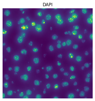
2. Plot the image

import numpy as np
import dask.array as da
from matplotlib.colors import Normalize

import matplotlib.pyplot as plt

fig, ax = plt.subplots(1, 1, figsize=(4, 4))
channel = "DAPI"
crd = [3000, 4000, 3000, 4000]  # crop is in pixel coordinates
to_coordinate_system = "pixel"

# normalization parameters for visualization (underlying image not changed)
# for visualization we normalize by the 99th percentile
se = hp.im.get_dataarray(sdata, element_name=image_name)
_channel_idx = np.where(se.c.data == channel)[0].item()
vmax = da.percentile(se.data[_channel_idx].flatten(), q=99).compute()
norm = Normalize(vmax=vmax, clip=False)

render_images_kwargs = {"cmap": "viridis", "norm": norm}
show_kwargs = {"title": channel, "colorbar": False}
ax = hp.pl.plot_sdata(
    sdata,
    image_name=image_name,
    channel=channel,
    crd=crd,
    to_coordinate_system=to_coordinate_system,
    render_images_kwargs=render_images_kwargs,
    show_kwargs=show_kwargs,
    ax=ax,
)
# frameless figure
ax.axis("off")

plt.tight_layout()
plt.show()

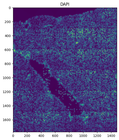
Or plot full image in micron coordinates:

fig, ax = plt.subplots(1, 1, figsize=(6, 6))
channel = "DAPI"
to_coordinate_system = "micron"

render_images_kwargs = {
    "cmap": "viridis",
    "norm": norm,
}
show_kwargs = {
    "title": channel,
    "colorbar": False,
}
ax = hp.pl.plot_sdata(
    sdata,
    image_name=image_name,
    channel=channel,
    crd=None,
    to_coordinate_system=to_coordinate_system,
    render_images_kwargs=render_images_kwargs,
    show_kwargs=show_kwargs,
    ax=ax,
)

plt.tight_layout()
plt.show()

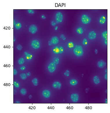
Queries can also be done in micron coordinates:

fig, ax = plt.subplots(1, 1, figsize=(4, 4))
channel = "DAPI"
crd = [400, 500, 400, 500]  # crops can also be specified in micron coordinates
to_coordinate_system = "micron"

render_images_kwargs = {"cmap": "viridis", "norm": norm}
show_kwargs = {"title": channel, "colorbar": False}
ax = hp.pl.plot_sdata(
    sdata,
    image_name=image_name,
    channel=channel,
    crd=crd,
    to_coordinate_system="micron",
    render_images_kwargs=render_images_kwargs,
    show_kwargs=show_kwargs,
    ax=ax,
)

plt.tight_layout()
plt.show()

3. Segment using Cellpose

import torch
from dask.distributed import Client, LocalCluster

if torch.cuda.is_available():
    from dask_cuda import LocalCUDACluster  # pip install dask-cuda

    # One worker per GPU; each worker will be pinned to a single GPU.
    cluster = LocalCUDACluster(
        CUDA_VISIBLE_DEVICES=[0],  # or [0,1],...etc
        n_workers=1,  # 2 if [0,1],...etc
        threads_per_worker=1,
        memory_limit="32GB",
        # local_directory=os.environ.get( "TMPDIR" ),#
    )
else:
    # cpu/mps fall back
    from dask.distributed import LocalCluster

    cluster = LocalCluster(
        n_workers=1
        if torch.backends.mps.is_available()
        else 8,  # If mps/cuda device available, it is better to increase chunk size to maximal value that fits on the gpu, and set n_workers to 1.
        # For this dummy example, we only have one chunk, so setting n_workers>1, has no effect.
        threads_per_worker=1,
        memory_limit="32GB",
        # local_directory=os.environ.get( "TMPDIR" ),
    )

client = Client(cluster)

print(client.dashboard_link)

sdata = hp.im.segment(
    sdata,
    image_name="raw_image",
    depth=200,
    model=hp.im.cellpose_callable,
    # parameters that will be passed to the callable cellpose_callable
    diameter=50,
    flow_threshold=0.9,
    cellprob_threshold=-4,
    output_labels_name="segmentation_mask",
    output_shapes_name="segmentation_mask_boundaries",
    crd=[
        3000,
        4000,
        3000,
        4000,
    ],  # region to segment [x_min, xmax, y_min, y_max], must be defined in pixel coordinates
    to_coordinate_system="pixel",
    overwrite=True,
)
client.close()

http://127.0.0.1:8787/status

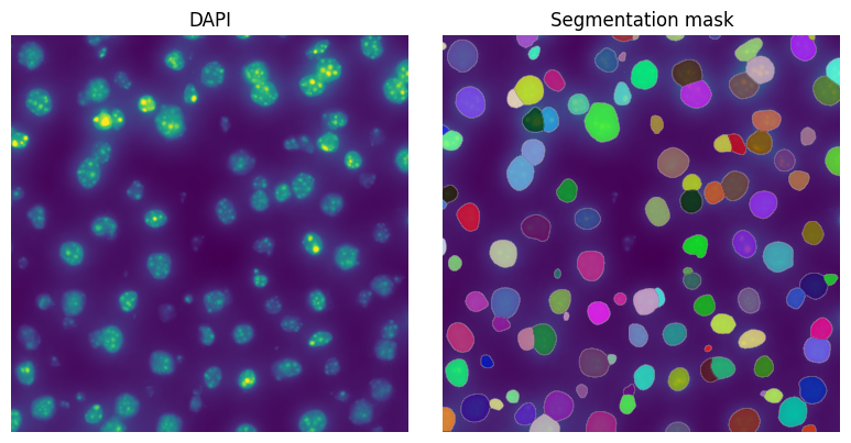
4. Visualize resulting segmentation

fig, axes = plt.subplots(1, 2, figsize=(8, 4))

channel = "DAPI"
image_name = "raw_image"
labels_name = "segmentation_mask"
crd = [
    3000,
    4000,
    3000,
    4000,
]  # Crop in pixels. One could also choose to do the crop in micron coordinates
to_coordinate_system = "pixel"

render_images_kwargs = {"cmap": "viridis", "norm": norm}
render_labels_kwargs = {"fill_alpha": 0.6, "outline_alpha": 0.4}
show_kwargs = {"title": channel, "colorbar": False}
_ax = hp.pl.plot_sdata(
    sdata,
    image_name=image_name,
    crd=crd,
    to_coordinate_system=to_coordinate_system,
    channel=channel,
    render_images_kwargs=render_images_kwargs,
    show_kwargs=show_kwargs,
    ax=axes[0],
)
_ax.axis("off")

show_kwargs = {"title": "Segmentation mask", "colorbar": False}
_ax = hp.pl.plot_sdata(
    sdata,
    image_name=image_name,
    labels_name=labels_name,
    crd=crd,
    to_coordinate_system=to_coordinate_system,
    channel=channel,
    render_images_kwargs=render_images_kwargs,
    render_labels_kwargs=render_labels_kwargs,
    show_kwargs=show_kwargs,
    ax=axes[1],
)
_ax.axis("off")

plt.tight_layout()
plt.show()

5. Read the transcripts

path_transcripts = registry.fetch(
    "transcriptomics/resolve/mouse/20272_slide1_A1-1_results.txt"
)
sdata = hp.io.read_resolve_transcripts(
    sdata,
    path_count_matrix=path_transcripts,
    output_points_name="transcripts",
    to_coordinate_system="pixel",
    to_micron_coordinate_system="micron",
    pixel_size=pixel_size,
    overwrite=True,
)
sdata

SpatialData object, with associated Zarr store: /private/var/folders/q5/7yhs0l6d0x771g7qdbhvkvmr0000gp/T/sdata_21e9705d-6c32-4296-b47c-b06327941efa.zarr
├── Images
│     └── 'raw_image': DataTree[cyx] (1, 12864, 10720), (1, 6432, 5360), (1, 3216, 2680), (1, 1608, 1340), (1, 804, 670)
├── Labels
│     └── 'segmentation_mask': DataArray[yx] (1000, 1000)
├── Points
│     └── 'transcripts': DataFrame with shape: (<Delayed>, 3) (2D points)
└── Shapes
      └── 'segmentation_mask_boundaries': GeoDataFrame shape: (121, 1) (2D shapes)
with coordinate systems:
    ▸ 'micron', with elements:
        raw_image (Images), segmentation_mask (Labels), transcripts (Points), segmentation_mask_boundaries (Shapes)
    ▸ 'pixel', with elements:
        raw_image (Images), segmentation_mask (Labels), transcripts (Points), segmentation_mask_boundaries (Shapes)

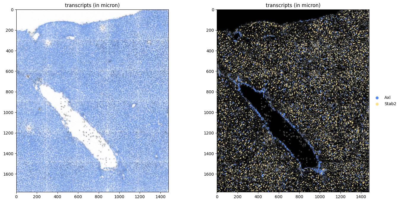
fig, axes = plt.subplots(1, 2, figsize=(16, 8))

render_images_kwargs = {
    "cmap": "binary",
}
show_kwargs = {
    "title": "transcripts (in micron)",
    "colorbar": False,
}

hp.pl.plot_sdata_genes(
    sdata,
    points_name="transcripts",
    image_name="raw_image",
    genes=None,  # plot all genes
    color="cornflowerblue",
    size=0.1,
    frac=0.5,  # only plot half of them
    to_coordinate_system="micron",
    show_kwargs=show_kwargs,
    render_images_kwargs=render_images_kwargs,
    ax=axes[0],
)

render_images_kwargs = {
    "cmap": "grey",
}
show_kwargs = {
    "title": "transcripts (in micron)",
    "colorbar": False,
}

hp.pl.plot_sdata_genes(
    sdata,
    points_name="transcripts",
    image_name="raw_image",
    genes=["Axl", "Stab2"],
    palette=["#4D88FF", "#FFE082"],
    size=5.0,
    frac=None,
    to_coordinate_system="micron",
    show_kwargs=show_kwargs,
    render_images_kwargs=render_images_kwargs,
    ax=axes[1],
)

INFO     Value for parameter 'color' appears to be a color, using it as such.
INFO     Using 'datashader' backend with 'None' as reduction method to speed up plotting. Depending on the         
         reduction method, the value range of the plot might change. Set method to 'matplotlib' do disable this    
         behaviour.
INFO     Using 'datashader' backend with 'None' as reduction method to speed up plotting. Depending on the         
         reduction method, the value range of the plot might change. Set method to 'matplotlib' do disable this    
         behaviour.

<Axes: title={'center': 'transcripts (in micron)'}>

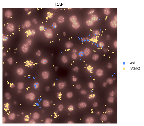
Or visualize a crop.

Querying points is slow in spatialdata, therefore, we query the points outside of spatialdata (and therefore also the image).

from spatialdata import bounding_box_query

crd = [3000, 4000, 3000, 4000]

to_coordinate_system = "pixel"  # we query in 'intrinsic' pixel coordinate system

y_start = crd[2]
x_start = crd[0]

y_end = crd[3]
x_end = crd[1]

name_x = "x"
name_y = "y"

y_query = f"{y_start} <={name_y} < {y_end}"
x_query = f"{x_start} <={name_x} < {x_end}"

query = f"{y_query} and {x_query}"

sdata["transcripts"] = sdata["transcripts"].categorize(columns=["gene"])
sdata["transcripts_queried"] = sdata["transcripts"].query(query)

sdata["raw_image_queried"] = bounding_box_query(
    sdata["raw_image"],
    axes=["x", "y"],
    min_coordinate=[crd[0], crd[2]],
    max_coordinate=[crd[1], crd[3]],
    target_coordinate_system=to_coordinate_system,
)

fig, axes = plt.subplots(1, 1, figsize=(6, 6))

render_images_kwargs = {
    "cmap": "pink",
}
show_kwargs = {
    "title": channel,
    "colorbar": False,
}

hp.pl.plot_sdata_genes(
    sdata,
    points_name="transcripts_queried",
    image_name="raw_image_queried",
    genes=["Axl", "Stab2"],
    palette=["#4D88FF", "#FFE082"],
    size=5.0,
    frac=None,
    crd=None,
    to_coordinate_system=to_coordinate_system,
    show_kwargs=show_kwargs,
    render_images_kwargs=render_images_kwargs,
    ax=axes,
)

del sdata["transcripts_queried"]
del sdata["raw_image_queried"]

axes.axis("off")

(np.float64(3000.0),
 np.float64(4000.0),
 np.float64(4000.0),
 np.float64(3000.0))

6. Create the AnnData table

# Use dask cluster for optimal processing. For this dummy example, one could also work without a dask cluster.
cluster = LocalCluster(
    n_workers=8,
    threads_per_worker=1,
    processes=True,
    memory_limit="8GB",
    # local_directory=os.environ.get( "TMPDIR" ),
)

client = Client(cluster)

print(client.dashboard_link)

http://127.0.0.1:49706/status

sdata = hp.tb.allocate(
    sdata,
    labels_name="segmentation_mask",
    points_name="transcripts",
    output_table_name="table_transcriptomics",
    chunks=None,
    to_coordinate_system="pixel",
    update_shapes_elements=False,
    overwrite=True,
)
sdata["table_transcriptomics"]

client.close()

sdata["table_transcriptomics"].to_df().head()

	Adamtsl2	Adgre1	Atp6v0d2	Axl	C5ar1	Ccr2	Cd207	Cd209a	Cd36	Cd3e	...	Sox9	Spn	Spon2	Stab2	Timd4	Tmem119	Vsig4	Vwf	Wnt2	Wnt9b
cells
65_segmentation_mask_a6baaa75	0	0	0	0	0	0	0	0	0	0	...	0	0	0	0	0	0	0	0	0	0
69_segmentation_mask_a6baaa75	0	0	0	0	0	0	0	0	0	0	...	0	0	0	0	0	0	0	0	0	0
71_segmentation_mask_a6baaa75	0	0	0	0	0	0	0	1	0	0	...	0	0	0	0	0	0	0	0	0	0
81_segmentation_mask_a6baaa75	0	0	0	0	0	0	0	0	0	0	...	0	0	0	0	0	0	0	0	0	0
83_segmentation_mask_a6baaa75	0	0	0	0	0	0	0	0	0	0	...	0	0	0	0	0	0	0	0	0	0

5 rows × 71 columns

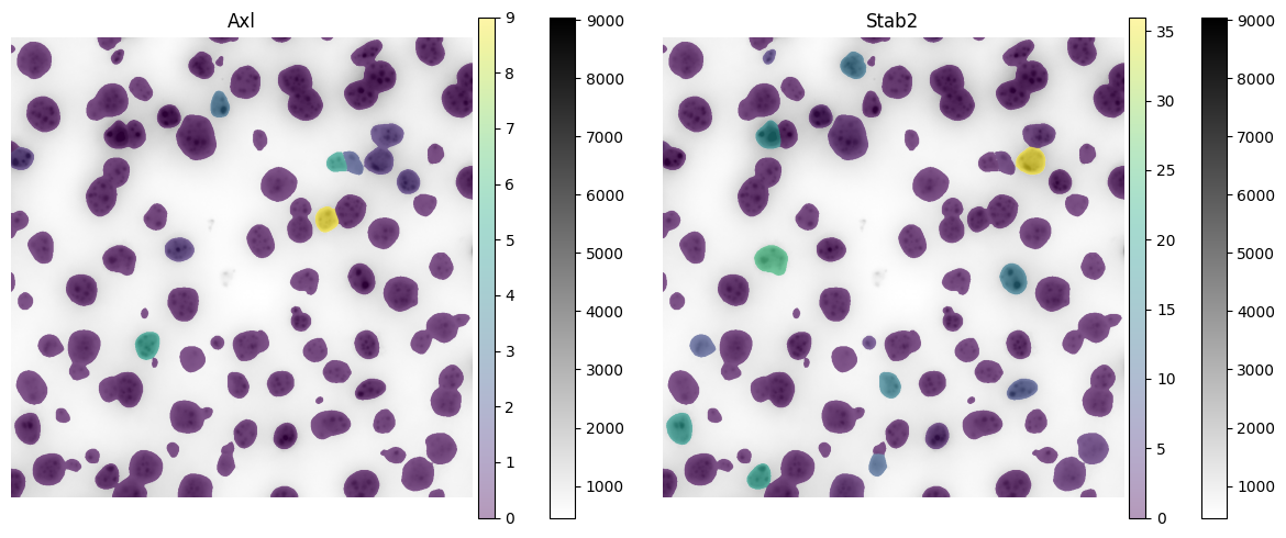
Now visualize the expression of 2 genes:

fig, axes = plt.subplots(1, 2, figsize=(12, 5))

channel = "DAPI"
image_name = "raw_image"
labels_name = "segmentation_mask"
table_name = "table_transcriptomics"
crd = [3000, 4000, 3000, 4000]
to_coordinate_system = "pixel"

render_images_kwargs = {"cmap": "binary", "norm": norm}
render_labels_kwargs = {"fill_alpha": 0.6, "outline_alpha": 0.4}

# subset because querying of points is slow, and we do not need them in this visualization
sdata_to_plot = sdata.subset(element_names=[image_name, labels_name, table_name])

color = "Axl"
show_kwargs = {
    "title": f"{color}",
    "colorbar": True,
}
ax = hp.pl.plot_sdata(
    sdata_to_plot,
    image_name=image_name,
    channel=channel,
    crd=crd,
    to_coordinate_system=to_coordinate_system,
    labels_name=labels_name,
    table_name=table_name,
    color=color,
    render_images_kwargs=render_images_kwargs,
    show_kwargs=show_kwargs,
    ax=axes[0],
)
ax.axis("off")

# color by mean intensity
color = "Stab2"
show_kwargs = {
    "title": f"{color}",
    "colorbar": True,
}
ax = hp.pl.plot_sdata(
    sdata_to_plot,
    image_name=image_name,
    channel=channel,
    crd=crd,
    to_coordinate_system=to_coordinate_system,
    labels_name=labels_name,
    table_name=table_name,
    color=color,
    render_images_kwargs=render_images_kwargs,
    show_kwargs=show_kwargs,
    ax=axes[1],
)
ax.axis("off")

plt.tight_layout()
plt.show()

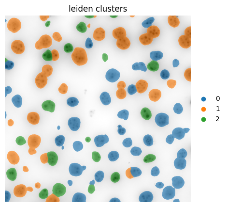
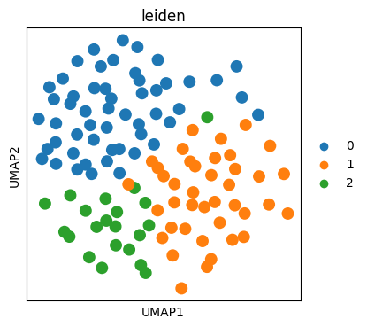
6. Leiden Clustering

sdata = hp.tb.preprocess_transcriptomics(
    sdata,
    labels_name="segmentation_mask",
    table_name="table_transcriptomics",
    output_table_name="table_transcriptomics_preprocessed",
    update_shapes_elements=False,
    overwrite=True,
)

sdata = hp.tb.leiden(
    sdata,
    labels_name="segmentation_mask",
    table_name="table_transcriptomics_preprocessed",
    output_table_name="table_transcriptomics_preprocessed",
    overwrite=True,
)

import scanpy as sc

fig, ax = plt.subplots(figsize=(4, 4))

sc.pl.umap(
    sdata["table_transcriptomics_preprocessed"],
    color="leiden",
    size=400,
    ax=ax,
)

fig, axes = plt.subplots(1, 1, figsize=(5, 5))

channel = "DAPI"
image_name = "raw_image"
labels_name = "segmentation_mask"
table_name = "table_transcriptomics_preprocessed"
crd = [3000, 4000, 3000, 4000]
to_coordinate_system = "pixel"

render_images_kwargs = {"cmap": "binary", "norm": norm}
render_labels_kwargs = {"fill_alpha": 0.6, "outline_alpha": 0.4}

# subset because querying of points is slow, and we do not need them in this visualization
sdata_to_plot = sdata.subset(element_names=[image_name, labels_name, table_name])

color = "leiden"
show_kwargs = {
    "title": f"{color} clusters",
    "colorbar": False,
}
ax = hp.pl.plot_sdata(
    sdata_to_plot,
    image_name=image_name,
    channel=channel,
    crd=crd,
    to_coordinate_system=to_coordinate_system,
    labels_name=labels_name,
    table_name=table_name,
    color=color,
    render_images_kwargs=render_images_kwargs,
    show_kwargs=show_kwargs,
    ax=axes,
)
ax.axis("off")

(np.float64(3000.0),
 np.float64(4000.0),
 np.float64(4000.0),
 np.float64(3000.0))